How Large Language Models Work — Part 1: Tokenization and Embeddings

This is Part 1 of a five-part deep-dive series on the internal mechanics of large language models. This series is written for engineers, ML practitioners, and technically advanced readers. Part 1 covers tokenization and embeddings — the first two stages through which raw text becomes a mathematical object a neural network can reason over.

Why Text Must Be Transformed

Neural networks are, at their core, mathematical functions that operate on tensors, which are multi-dimensional arrays of floating-point numbers. They cannot accept raw text strings as input. Before a language model can do anything useful, it must convert a sequence of characters into a sequence of numbers. This two-step process of tokenization followed by embedding is where all LLM processing begins, and understanding it deeply is prerequisite to understanding everything that follows.

Stage 1: Tokenization

What a Tokenizer Does

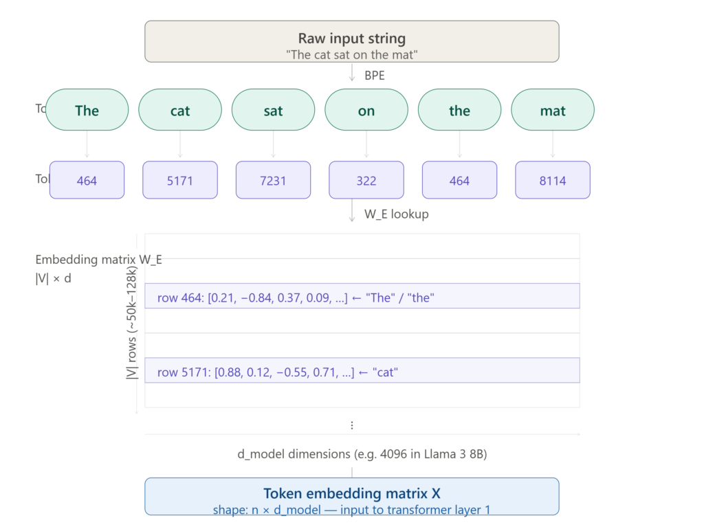
A tokenizer breaks a raw string into a sequence of discrete units called tokens, and maps each token to an integer index in a fixed vocabulary. Given the input string:

"The cat sat on the mat"

a tokenizer might produce the token sequence: [464, 5171, 7231, 322, 464, 8114]

Each integer is an index into a vocabulary table of size $|V|$, typically between 32,000 and 100,000 entries for modern models. GPT-4 uses a vocabulary of approximately 100,277 tokens. Llama 3 uses 128,256.

Byte-Pair Encoding (BPE)

The dominant tokenization algorithm used in modern LLMs is Byte-Pair Encoding (BPE), originally a data compression algorithm adapted for NLP by Sennrich et al. in 2016.

BPE builds its vocabulary through an iterative merging process:

1. Initialise the vocabulary with every individual character (or byte) in the training corpus.
2. Count all adjacent symbol pairs across the corpus.
3. Merge the most frequent pair into a single new symbol.
4. Repeat steps 2–3 until the vocabulary reaches the target size $|V|$∣V∣.

The result is a vocabulary that contains individual characters, common subwords, and frequent whole words. The word “tokenization” might be represented as three tokens: token, ization is further split into iz, ation depending on training corpus frequency.

This has a critical practical consequence: no word is ever truly unknown to a BPE tokenizer. Any string, including code, URLs, foreign scripts, or novel proper nouns, can be decomposed into its constituent bytes if nothing else matches. This is why BPE-based models generalise to inputs they have never seen verbatim.

Token Fertility and Efficiency

Not all languages tokenize equally efficiently. English text typically tokenizes at roughly 0.75 tokens per word. Languages with richer morphology, such as Finnish, Turkish, Arabic, or non-Latin scripts, tokenize less efficiently, sometimes requiring 3–5 tokens per word. This has practical implications: a context window of 128,000 tokens holds far more English prose than it does Thai or Arabic text, a bias baked into the model’s architecture from the vocabulary construction stage.

The fertility of a tokenizer, or the average number of tokens per word, is a meaningful measure of how well it serves a given language or domain. Code-optimised models like DeepSeek Coder use vocabularies with explicit code tokens to reduce the fertility of common programming constructs.

WordPiece and SentencePiece

Two notable alternatives to BPE are worth knowing:

WordPiece, used in BERT and its derivatives, is similar to BPE but merges pairs that maximise the likelihood of the training data under a language model, rather than simply the most frequent pair. This produces slightly different vocabulary distributions.

SentencePiece, used in models including Llama and T5, treats the input as a raw unicode byte stream with no pre-tokenization step (no whitespace splitting). This makes it language-agnostic and particularly well-suited for multilingual models.

Stage 2: Token Embeddings

The Embedding Matrix

Once tokenization has produced a sequence of integer indices $[t_1, t_2, \ldots, t_n]$, each index must be converted into a dense vector. This is done via an embedding matrix $W_E \in \mathbb{R}^{|V| \times d}$, where $d$ is the model’s hidden dimension (also called the embedding dimension or $d_{\text{model}}$​).

The embedding for token $t_i$ti​ is simply a row lookup:$$\mathbf{e}_i = W_E[t_i] \in \mathbb{R}^d$$In GPT-3, $d = 12288$. In Llama 3 8B, $d = 4096$. This single matrix, learned entirely from data during pre-training, is responsible for encoding the semantic relationships between all tokens in the vocabulary.

The number of parameters in the embedding matrix alone is $|V| \times d$. For GPT-4’s approximate configuration, that is $100{,}277 \times d_{\text{model}}$ which is often hundreds of millions of parameters just for this one component.

Why Dense Vectors Work: The Geometry of Meaning

The remarkable property of learned embeddings is that semantic relationships emerge as geometric relationships in $\mathbb{R}^d$. The classic demonstration is the linear analogy:

$$\mathbf{e}(\text{“king”}) – \mathbf{e}(\text{“man”}) + \mathbf{e}(\text{“woman”}) \approx \mathbf{e}(\text{“queen”})$$

This is not programmed. It emerges from the statistical structure of co-occurrence patterns in the training corpus. Words that appear in similar contexts end up with similar embedding vectors, measured by cosine similarity:$$\text{sim}(\mathbf{u}, \mathbf{v}) = \frac{\mathbf{u} \cdot \mathbf{v}}{\|\mathbf{u}\| \|\mathbf{v}\|}$$In high-dimensional spaces, this geometry becomes extraordinarily rich. Directions in embedding space can encode syntactic roles, semantic fields, sentiment polarities, and factual associations — all simultaneously, in different orthogonal subspaces of the same $\mathbb{R}^d$.

Stage 3: Positional Encoding

Token embeddings encode what each token is, but they contain no information about where in the sequence each token appears. The sequence "dog bites man" and "man bites dog" would produce identical sets of token embeddings in a different order and would be catastrophic for a model that needs to understand syntax and word order.

Positional information must therefore be injected explicitly.

Sinusoidal Positional Encoding (Original Transformer)

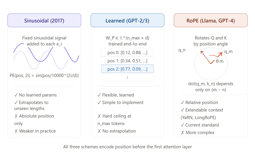
The original transformer paper (Vaswani et al., 2017) proposed adding a fixed sinusoidal signal to each token embedding. For position $pos$pos and dimension $i$i:$$PE_{(pos, 2i)} = \sin\!\left(\frac{pos}{10000^{2i/d}}\right)$$ $$PE_{(pos, 2i+1)} = \cos\!\left(\frac{pos}{10000^{2i/d}}\right)$$

The input to the first transformer layer is then:$$\mathbf{x}_i = \mathbf{e}_i + PE_i$$

The sinusoidal formulation has a useful property: the positional encoding of position $pos + k$ can be expressed as a linear function of the encoding at $pos$pos, which makes it easy for attention heads to learn to attend to tokens at a fixed relative offset.

Learned Positional Embeddings

GPT-2 and GPT-3 replaced sinusoidal encodings with learned positional embeddings: a second matrix $W_P \in \mathbb{R}^{n_{\text{max}} \times d}$​, where $n_{\text{max}}$​ is the maximum context length. Position $pos$pos adds the row $W_P[pos]$ to the token embedding. These are learned end-to-end during pre-training and tend to slightly outperform sinusoidal encodings on benchmarks, at the cost of a hard context length ceiling — the model cannot generalise beyond $n_{\text{max}}$​ positions it has seen during training.

Rotary Positional Embedding (RoPE)

The current state of the art for most frontier models, including Llama, Mistral, GPT-4, and Gemini, is Rotary Positional Embedding (RoPE), introduced by Su et al. in 2021.

Rather than adding a positional vector to the token embedding, RoPE encodes position by rotating the Query and Key vectors in the attention mechanism (covered in Part 2) by a position-dependent angle. For a vector at position $m$m in dimension pair $(2i, 2i+1)$:$$\mathbf{q}_m^{(i)} = \begin{pmatrix} q_{2i} \\ q_{2i+1} \end{pmatrix} \begin{pmatrix} \cos m\theta_i & -\sin m\theta_i \\ \sin m\theta_i & \cos m\theta_i \end{pmatrix}$$

where $\theta_i = 10000^{-2i/d}$.

The critical advantage: the dot product between a query at position $m$m and a key at position $n$n depends only on their relative offset $m – n$, not their absolute positions. This gives the model a natural inductive bias toward relative position awareness, and with extensions like YaRN makes it possible to extend the effective context window well beyond what the model was trained on.

RoPE is why modern models can be fine-tuned to handle 128K or even 1M token context windows without retraining the entire model from scratch.

Putting It Together: The Input Representation

The final input to the first transformer layer for a sequence of $n$n tokens is a matrix $X \in \mathbb{R}^{n \times d}$:$$X = \begin{pmatrix} \mathbf{e}_1 + \mathbf{p}_1 \\ \mathbf{e}_2 + \mathbf{p}_2 \\ \vdots \\ \mathbf{e}_n + \mathbf{p}_n \end{pmatrix}$$where $\mathbf{p}_i$ is the positional encoding for position $i$ (sinusoidal, learned, or RoPE-derived). Each row of $X$ is a $d$-dimensional vector carrying both the semantic identity of the token and its position in the sequence. This matrix is what flows into the self-attention mechanism, which is the subject of Part 2.

---

Key Numbers to Anchor Your Intuition

Model	Vocabulary $\|V\|$	$d_{\text{model}}$	Positional scheme
GPT-2	50,257	768–1,600	Learned
GPT-3	50,257	12,288	Learned
Llama 3 8B	128,256	4,096	RoPE
Mistral 7B	32,000	4,096	RoPE
Gemma 2	256,000	2,304–3,584	RoPE

---

Conclusion

Before a single attention head fires, a large language model has already done substantial mathematical work. A raw string has been segmented into subword tokens by a BPE or SentencePiece algorithm, each token has been projected into a high-dimensional vector space where geometry encodes meaning, and position information has been woven in either additively or, in modern models, rotationally via RoPE. The quality of this input representation has an outsized effect on everything downstream: models with poorly constructed vocabularies or weak embedding initialisations are harder to train and less capable at convergence.

Part 2 will take this matrix $X \in \mathbb{R}^{n \times d}$ and walk through exactly what the self-attention mechanism does with it, including the full mathematical derivation of scaled dot-product attention, multi-head attention, and what different heads actually learn to represent.

Coming next in the AI Engineering series is Part 2: The Attention Mechanism.