How Large Language Models Work — Part 3: The Transformer Block and Architecture

This is Part 3 of a five-part series on the internal mechanics of large language models. Part 2 derived scaled dot-product attention and the KV cache. Part 3 traces the complete transformer block consisting of feed-forward networks, layer normalisation, and residual streams; it examines the architectural differences between decoder-only and encoder-decoder models.

From Attention Output to Transformer Block

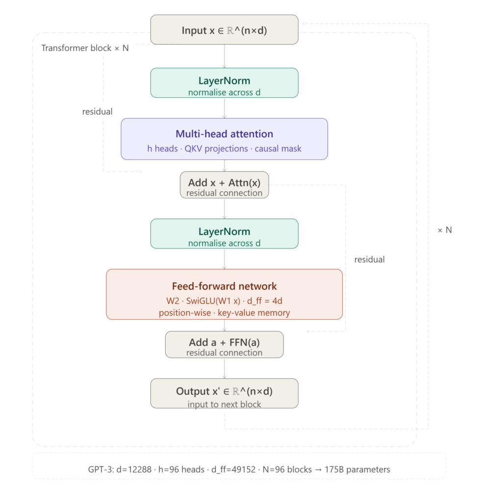
At the end of Part 2, self-attention had produced an output matrix $O \in \mathbb{R}^{n \times d}$ or one updated vector per token, now containing contextual information drawn from every other position in the sequence. But this is only the first half of a single transformer block. Before the signal moves to the next layer, it passes through three more components: a residual connection, layer normalisation, and a position-wise feed-forward network. Together with multi-head attention, these four elements constitute the repeating unit of every transformer-based LLM, stacked $N$ times to form the full model.

Understanding each component precisely is important not just for implementation, but for diagnosing failure modes, interpreting mechanistic interpretability research, and making informed decisions about architectural variants when selecting or fine-tuning models.

Residual Connections

The residual connection, introduced in ResNets for computer vision and adopted into transformers from the outset, is deceptively simple. Rather than passing the attention output $O$ directly to the next component, the original input $X$ is added back:$$X’ = X + \text{MultiHead}(X)$$

This addition of the residual or skip connection has several important consequences.

First, it solves the vanishing gradient problem for very deep networks. During backpropagation, gradients flow backward through the network. Without residual connections, multiplying many Jacobians together through $N$N sequential non-linear transformations causes gradient magnitudes to decay exponentially, making early layers extremely slow to learn. The residual path provides a direct gradient highway that bypasses each block, so that gradients can flow backward through the addition operation unchanged, regardless of how many layers separate the loss from the input.

Second, and more subtly, residual connections give the network an inductive bias toward learning incremental transformations. Rather than learning to reconstruct the full representation from scratch at each layer, each block learns only the delta or the correction to add to the existing representation. In mechanistic interpretability, researchers conceptualise the transformer as a residual stream: a $d$-dimensional vector that is progressively written to and read from by successive attention heads and feed-forward layers, each contributing small structured updates. This framing, developed extensively by Anthropic, EleutherAI, and Neel Nanda’s research group, has proven highly productive for understanding what specific components of large models actually compute.

Layer Normalisation

Before and/or after each sub-component, layer normalisation is applied. For a vector $\mathbf{x} \in \mathbb{R}^d$:$$\text{LayerNorm}(\mathbf{x}) = \gamma \odot \frac{\mathbf{x} – \mu}{\sigma + \epsilon} + \beta$$

where $\mu = \frac{1}{d}\sum_i x_i$ is the mean, $\sigma = \sqrt{\frac{1}{d}\sum_i (x_i – \mu)^2}$ is the standard deviation, $\epsilon$ is a small constant for numerical stability, and $\gamma, \beta \in \mathbb{R}^d$ are learned scale and shift parameters.

Layer normalisation stabilises training by preventing the internal covariate shift problem, which is the tendency for the distribution of a layer’s inputs to change as upstream parameters update, forcing each layer to continuously readapt. By normalising each token’s representation independently across the feature dimension (as opposed to batch normalisation, which normalises across the batch dimension), layer norm is compatible with variable-length sequences and works correctly with batch size 1, making it well-suited for autoregressive inference.

Two conventions exist for where layer norm is placed within the block:

Post-norm (original Transformer, “Attention Is All You Need”): LayerNorm is applied after the residual addition:$$X’ = \text{LayerNorm}(X + \text{MultiHead}(X))$$

Pre-norm (GPT-2, GPT-3, most modern LLMs): LayerNorm is applied to the input before the sub-component:$$X’ = X + \text{MultiHead}(\text{LayerNorm}(X))$$

Pre-norm has become the dominant convention because it produces more stable training dynamics at large scale. Gradients flow more cleanly through the unmodified residual path, and the model is less sensitive to initialisation and learning rate choice. The architectural difference is subtle but has meaningful empirical consequences; models trained with post-norm often require careful learning rate warmup schedules that pre-norm models do not.

The Feed-Forward Network

After the attention sub-layer (with its own residual connection and layer norm), each transformer block applies a position-wise feed-forward network (FFN). The term “position-wise” means the same two-layer MLP is applied independently to each token’s vector, and the FFN has no cross-token interactions, unlike attention.

The standard formulation:$$\text{FFN}(\mathbf{x}) = W_2 \cdot \sigma(W_1 \mathbf{x} + \mathbf{b}_1) + \mathbf{b}_2$$

where $W_1 \in \mathbb{R}^{d_{\text{ff}} \times d}$, $W_2 \in \mathbb{R}^{d \times d_{\text{ff}}}$​, and $d_{\text{ff}}$​ is the intermediate dimension, typically $4d$. In GPT-3, $d = 12288$ and $d_{\text{ff}} = 49152$, giving each FFN roughly $4 \times 12288^2 \approx 603$ million parameters, more than the attention sub-layer at that layer.

The activation function $\sigma$σ has evolved across generations. The original transformer used ReLU. GPT-2 and GPT-3 used GeLU (Gaussian Error Linear Unit), which approximates ReLU with a smooth, non-zero gradient for slightly negative inputs:$$\text{GeLU}(x) = x \cdot \Phi(x) \approx 0.5x\!\left(1 + \tanh\!\left(\sqrt{\frac{2}{\pi}}\left(x + 0.044715x^3\right)\right)\right)$$

where $\Phi$ is the standard normal CDF. More recent models use SwiGLU, a gated variant introduced by Noam Shazeer in 2020 and adopted in PaLM, Llama, and most frontier models:$$\text{SwiGLU}(\mathbf{x}) = \text{SiLU}(W_1 \mathbf{x}) \odot (W_3 \mathbf{x})$$

where $\text{SiLU}(x) = x \cdot \sigma(x)$ is the Sigmoid Linear Unit and $W_3$​ is an additional learned gate projection. SwiGLU consistently outperforms GeLU on downstream benchmarks, though the underlying reason remains an active area of research. When using SwiGLU, $d_{\text{ff}}$​ is typically set to $\frac{8}{3}d$ rather than $4d$ to keep parameter counts comparable across architectures.

What does the FFN actually learn? Mechanistic interpretability work, particularly from Anthropic and the Neel Nanda group, has provided strong evidence that FFN layers function as key-value memories. Each row of $W_1$​ acts as a pattern detector (a “key”), and the corresponding row of $W_2$ stores an associated “value” that gets added to the residual stream when that pattern is detected. This explains why larger FFNs improve factual recall (they have more memory slots) and why deleting specific FFN neurons can surgically remove specific factual associations from a model’s behaviour.

The Complete Transformer Block

Assembling all components, the full pre-norm transformer block for a decoder-only model is:$$\mathbf{a} = \mathbf{x} + \text{MultiHead}(\text{LayerNorm}(\mathbf{x}))$$ $$\mathbf{x}’ = \mathbf{a} + \text{FFN}(\text{LayerNorm}(\mathbf{a}))$$

This two-step computation, attention followed by FFN, each with its own pre-norm and residual, is repeated $N$ times. In GPT-3, $N = 96$. In Llama 3 70B, $N = 80$. In a typical GPT-4-class model, $N$ is believed to be in the range of 96–120 layers. Each repetition allows the model to build increasingly abstract representations. Early layers handle low-level syntactic patterns, while later layers encode semantic and factual content.

Decoder-Only vs Encoder-Decoder Architecture

Two principal transformer architectures are in widespread use, differing in how they process input and generate output.

Decoder-only models (GPT, Llama, Mistral, Gemma, Falcon) use a single stack of transformer blocks with causal (masked) self-attention. Every token can attend only to previous tokens. The entire input prompt and the generated output share the same context window and are processed by the same stack. At inference time, the model autoregressively generates one token at a time, each conditioned on all prior tokens. This architecture is dominant for general-purpose language models because it scales efficiently and the training objective of next-token prediction across the entire sequence is simple, scalable, and empirically powerful.

Encoder-decoder models (T5, BART, mT5, the original Transformer for machine translation) use two distinct stacks. The encoder processes the full input with bidirectional attention. Every token can attend to every other token simultaneously, with no causal mask. The encoded representation is then passed to the decoder via a cross-attention mechanism: each decoder token’s query attends to the encoder’s key-value pairs in addition to previously generated decoder tokens. The cross-attention block takes the form:$$\text{CrossAttn}(Q_{\text{dec}},\ K_{\text{enc}},\ V_{\text{enc}}) = \text{softmax}\!\left(\frac{Q_{\text{dec}} K_{\text{enc}}^\top}{\sqrt{d_k}}\right)V_{\text{enc}}$$

This architecture was originally designed for sequence-to-sequence tasks such as translation, summarisation, or question answering, where the full input is available before generation begins. It has largely been supplanted by decoder-only models for general language tasks, primarily because the instruction-tuned decoder-only paradigm proved more flexible and scalable. However, encoder-decoder models retain advantages for tasks requiring deep understanding of a fixed input, such as structured prediction, constrained generation, and certain retrieval tasks.

A hybrid, the encoder-only model (BERT, RoBERTa, DeBERTa), uses bidirectional attention with no autoregressive generation. It is optimised for discriminative tasks such as classification, named entity recognition, or semantic similarity, rather than generation, and remains widely used in production embedding pipelines and retrieval systems.

Depth, Width, and the Scaling Hypothesis

The transformer block’s design raises a natural question: does it matter whether a model has more layers (depth) or larger hidden dimension (width)? Empirically, the two interact in complex ways, and the optimal allocation of a fixed parameter budget between depth and width is one of the central questions addressed by scaling law research, which is the subject of Part 4.

What is clear from both theory and experiment is that depth and width serve different functions. Width increases the model’s representational capacity at each layer by the size of the residual stream and the richness of the key-value memory in the FFN. Depth increases the number of sequential computational steps the model can take, which means the number of times attention and FFN transformations can be composed. Tasks requiring multi-step reasoning appear to benefit disproportionately from depth, while factual recall scales more uniformly with total parameter count regardless of how it is distributed between depth and width.

Conclusion

The transformer block is elegant in its modularity: a residual stream, two sub-components (attention and FFN), and two layer normalisation steps. The full model is simply this block repeated $N$ times. But the interactions between these components, including the gradient flow through residual connections, the factual storage in FFN key-value memories, and the progressive abstraction through depth, give rise to capabilities that are not predictable from any single component in isolation.

Part 4 will move from architecture to training: the next-token prediction objective, loss functions, the Chinchilla scaling laws, and the dramatic effect of RLHF and instruction tuning on model behaviour, explaining why InstructGPT, at a fraction of GPT-3’s parameter count, consistently outperformed it.

Coming next in the AI Engineering series is Part 4: Training, Scaling Laws, and RLHF.