Complete RAG Pipelines from Scratch in 4 Steps: Chunking, Embedding, and Retrieval

The Problem RAG Solves

Do you want to learn how to build a RAG Pipeline from Scratch? Every large language model has a knowledge cutoff. It knows what it was trained on, and nothing beyond that. Ask a frontier model about a document it has never seen, a database record updated this morning, or a policy that changed last week, and it will either hallucinate an answer or tell you it does not know. For the vast majority of real enterprise AI applications, this is a fundamental limitation.

Retrieval-Augmented Generation (RAG) solves it. Rather than relying solely on what is baked into the model’s weights, RAG retrieves relevant content from an external knowledge source at query time and injects it into the model’s context window before generation. The model now has access to specific, current, verifiable information when it generates its answer. The result is a system that combines the reasoning capability of a frontier model with the factual grounding of a real knowledge base.

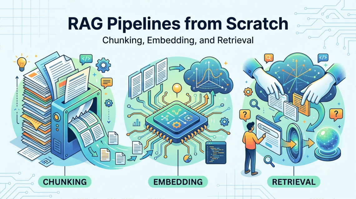
Building a RAG pipeline from scratch requires understanding three distinct stages: chunking the source documents into retrievable units, embedding those chunks into a vector space, and retrieving the right chunks at query time. Each stage has engineering decisions that significantly affect the quality of the final system.

Stage 1: Chunking

Chunking is the process of splitting source documents into smaller pieces that can be individually embedded and retrieved. It sounds simple, but it is where many RAG pipelines fail silently.

The core tension in chunking is between specificity and context. Small chunks are precise: a retrieval system can return exactly the passage relevant to a query without padding. But small chunks lose surrounding context, which means the model may receive a fragment that is accurate but uninterpretable without the sentences around it. Large chunks preserve context but dilute relevance: the retrieved passage contains the answer plus a lot of surrounding material that consumes precious context window tokens without contributing to the response.

Fixed-size chunking splits documents by token or character count, typically 256 to 512 tokens per chunk, with an overlap of 10 to 20 percent between adjacent chunks. The overlap ensures that sentences spanning a chunk boundary are represented fully in at least one chunk. This approach is fast, predictable, and easy to implement:

def fixed_size_chunks(text: str,
                      chunk_size: int = 512,
                      overlap: int = 64) -> list[str]:
    tokens = tokenizer.encode(text)
    chunks = []
    start = 0
    while start < len(tokens):
        end = min(start + chunk_size, len(tokens))
        chunks.append(tokenizer.decode(tokens[start:end]))
        start += chunk_size - overlap
    return chunks

Semantic chunking splits on natural boundaries: paragraphs, sections, or sentences, then merges adjacent units until a target size is reached. This preserves the logical structure of the document far better than fixed-size splitting and is the preferred approach for documents with clear section structure such as contracts, technical documentation, and research papers.

Hierarchical chunking maintains both a summary chunk and detailed sub-chunks for each section. At retrieval time, the system first retrieves summary-level chunks to identify the right section, then drills down to the detailed chunks within it. This approach produces significantly better results on long documents but requires more complex indexing infrastructure.

A practical rule: for structured documents such as PDFs, legal text, and technical manuals, use semantic chunking. For conversational logs, emails, and unstructured text, fixed-size chunking with generous overlap is typically sufficient. Always add metadata to each chunk: the source document name, page number, section heading, and creation date. This metadata is invaluable for filtering at retrieval time and for attributing sources in the final response.

Stage 2: Embedding

Once documents are chunked, each chunk must be converted into a dense vector that captures its semantic meaning. This is done using an embedding model: a neural network trained to map text into a high-dimensional space where semantically similar passages are geometrically close to each other.

The choice of embedding model matters significantly. The dominant options in 2026 are OpenAI’s text-embedding-3-large (3,072 dimensions), Cohere’s embed-v3, and open-source alternatives such as bge-large-en-v1.5 from BAAI and e5-mistral-7b-instruct from Microsoft. Open-source models have the advantage of running locally, which matters for data-sensitive applications.

Embedding a corpus in Python using the OpenAI API looks like this:

from openai import OpenAI
import numpy as np

client = OpenAI()

def embed_chunks(chunks: list[str],
                 model: str = "text-embedding-3-large") -> np.ndarray:
    response = client.embeddings.create(
        input=chunks,
        model=model
    )
    return np.array([item.embedding for item in response.data])

Two practical considerations deserve attention here. First, embed your queries using the same model you used to embed your documents. Mixing embedding models produces meaningless similarity scores because the vector spaces are incompatible. Second, normalise your embedding vectors before storing them if you plan to use cosine similarity for retrieval: most vector databases do this automatically, but it is worth verifying.

For domain-specific applications, fine-tuning an embedding model on in-domain data consistently outperforms general-purpose embeddings. A legal RAG system fine-tuned on case law retrieves significantly more relevant passages than a general embedding model applied to the same corpus, because the fine-tuned model learns the specific vocabulary and semantic relationships of the domain.

Stage 3: Vector Storage

Embeddings must be stored in a system that supports efficient similarity search. The options divide into three categories.

Dedicated vector databases such as Pinecone, Weaviate, Qdrant, and Milvus are purpose-built for high-dimensional vector search. They support filtering on metadata, approximate nearest-neighbour (ANN) search algorithms such as HNSW (Hierarchical Navigable Small World), and horizontal scaling to billions of vectors. For production systems with large corpora, these are the right choice.

Hybrid stores such as pgvector (a PostgreSQL extension) allow vector search within an existing relational database. This is useful when you want to combine semantic search with SQL filtering in a single query, which is a common pattern for structured data sources.

In-memory search using libraries such as FAISS or Annoy is suitable for development, prototyping, and small corpora where latency is critical and persistence is not required.

import faiss
import numpy as np

def build_faiss_index(embeddings: np.ndarray) -> faiss.IndexFlatIP:
    dimension = embeddings.shape[1]
    index = faiss.IndexFlatIP(dimension)  # inner product = cosine on normalised vectors
    faiss.normalize_L2(embeddings)
    index.add(embeddings)
    return index

Stage 4: Retrieval

At query time, the user’s question is embedded using the same model used to embed the documents, and the vector store is queried for the most similar chunks. This is where several common RAG pipeline failures occur, and where the most productive engineering improvements can be made.

Naive top-k retrieval returns the k most similar chunks by cosine similarity. It is a good starting point but has two well-known weaknesses. First, it relies entirely on the query embedding capturing the user’s intent accurately, which fails when queries are vague or use different terminology from the source documents. Second, the top-k chunks may all be from the same section of the same document, producing redundant context rather than diverse coverage.

Hybrid retrieval combines semantic (vector) search with keyword (BM25) search and merges the results using Reciprocal Rank Fusion (RRF). This is the most reliably effective retrieval strategy for general-purpose RAG and is now the default approach in most production systems. Keyword search catches exact term matches that semantic search misses; semantic search catches paraphrases and conceptual matches that keyword search misses.

Query rewriting passes the user’s query through the LLM before retrieval, expanding it into multiple alternative phrasings or decomposing a complex question into simpler sub-queries. Each sub-query is retrieved separately, and the results are merged before generation. This significantly improves retrieval quality on complex, multi-part questions.

Re-ranking adds a second-pass model after initial retrieval. A cross-encoder model such as Cohere Rerank or a locally hosted BGE re-ranker scores each retrieved chunk against the original query more accurately than the bi-encoder embedding similarity used in the initial retrieval, and re-orders the results accordingly. Re-ranking consistently improves answer quality at the cost of an additional model call.

Putting It Together

A minimal but complete RAG pipeline in production should: chunk documents semantically with metadata, embed with a domain-appropriate model, store in a vector database with metadata filtering, retrieve using hybrid search with re-ranking, and inject the retrieved context into a well-structured prompt with source attribution. Each of these steps is independently tunable, which means RAG pipeline quality can be improved incrementally without retraining the underlying LLM.

The engineering value of RAG is precisely this modularity. The knowledge base can be updated without touching the model. The retrieval strategy can be improved without reindexing. The generation model can be swapped without rebuilding the index. That separation of concerns is what makes RAG the most widely deployed pattern in production AI engineering today.