Inside the Data Processing Layer: Part 2, The Complete Data Analytics Stack

This is Part 2 of a three-part series on the modern data analytics stack. Part 1 covered sources, ingestion, and storage. Part 2 covers the data processing layer itself, transformation, and modeling. Part 3 will cover visualization, deployment, and orchestration.

Where Raw Data Becomes Useful Data

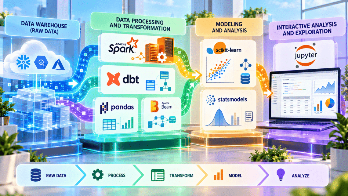
Part 1 of this series ended with data sitting in a warehouse, stored and queryable but still essentially raw. The data processing layer is where that raw material gets shaped into something an analyst, a model, or a dashboard can actually consume. This article goes deep into the specific engineering behind Spark, dbt, Pandas, and the analysis tools that sit downstream of them.

Apache Spark: Distributed Computation at Scale

Apache Spark sits at the center of the modern data processing layer for one specific reason. It solves the problem of processing datasets too large to fit in a single machine’s memory, by distributing computation across a cluster of machines working in parallel.

The core abstraction underlying Spark is the Resilient Distributed Dataset, or RDD. An RDD is a fault-tolerant collection of records, partitioned across the cluster, that Spark can rebuild automatically if a node fails, by replaying the sequence of transformations that created it rather than storing full data replicas. This lineage-based recovery is what gives Spark its resilience without the storage overhead of constant replication.

Spark’s real performance advantage over older systems like Hadoop MapReduce comes from a specific architectural choice. In-memory computation. MapReduce writes intermediate results to disk between every single processing stage, incurring expensive disk I/O repeatedly throughout a job. Spark instead keeps intermediate data in memory across stages whenever possible, only spilling to disk when memory genuinely runs out. For iterative workloads, the kind common in machine learning training, this difference compounds dramatically, since the same dataset gets read and processed multiple times across training iterations.

Spark also uses lazy evaluation. Transformations like map or filter do not execute immediately when called. Instead, Spark builds a Directed Acyclic Graph, or DAG, of the full computation plan, and only executes it when an action, something that actually requires a result, like count or collect, gets triggered. This laziness lets Spark’s Catalyst optimizer examine the entire planned computation before running anything, reordering operations and eliminating unnecessary work for genuinely faster execution.

dbt: Transformation as Software Engineering

dbt, short for data build tool, represents a philosophical shift in how the data processing layer handles transformation logic. Rather than writing custom Python or Scala transformation code, dbt lets analysts write transformations as SQL SELECT statements, then compiles and runs them directly inside the warehouse itself, using the warehouse’s own compute engine.

The technical innovation here is dbt’s dependency graph, built automatically from ref() function calls inside each model file. When one SQL model references another through ref(), dbt parses these references to construct a full DAG of the entire transformation pipeline, then executes models in the correct topological order, ensuring every dependency runs before anything that depends on it.

dbt also introduces materialization strategies, which control exactly how a given transformation gets persisted. A view materialization creates a virtual table, recomputed fresh on every query, using zero storage but costing compute every time it runs. A table materialization physically stores the full result, trading storage cost for consistently fast query performance. An incremental materialization processes only new or changed records since the last run, tracked through a specified unique key, dramatically reducing compute cost for very large, slowly changing datasets. Choosing the correct materialization strategy for each specific model is one of the most consequential technical decisions inside a real dbt-driven data processing layer.

Pandas and the Single-Machine Ceiling

Pandas remains the default tool for a huge share of exploratory data work, precisely because its DataFrame abstraction maps intuitively onto how analysts think about tabular data. Technically, Pandas builds on NumPy arrays underneath, giving it fast, vectorized operations that avoid Python’s notoriously slow native loops by pushing computation down into optimized, compiled C code.

The critical limitation to understand is memory. Pandas operates entirely in a single machine’s RAM. A DataFrame larger than available memory will simply fail, or degrade catastrophically through excessive disk swapping. This is precisely why the data processing layer in real production systems routes large-scale transformation through Spark first, then hands off a reduced, aggregated dataset to Pandas only once it is small enough to fit comfortably in memory for final, detailed analysis.

Apache Beam: One API, Multiple Execution Engines

Apache Beam addresses a specific architectural pain point. Portability across processing engines. Beam provides a unified programming model for both batch and streaming data, expressed through Pipelines, PCollections, and PTransforms, that can then execute on multiple different backend runners, including Spark, Google Cloud Dataflow, or Apache Flink, without rewriting the underlying pipeline logic.

Beam’s windowing model deserves particular attention for streaming workloads within the data processing layer. Since streaming data has no natural endpoint, Beam introduces the concept of windows, finite time-based groupings of otherwise infinite data, alongside watermarks, which estimate how complete the data within a given window actually is, and triggers, which determine exactly when to emit results for a window that may still be receiving late-arriving data. This combination lets Beam handle the genuinely hard problem of producing accurate, timely aggregations from data streams where individual records can arrive late, out of order, or delayed by network conditions.

The Modeling Layer: scikit-learn and Statsmodels

Once data has been processed and transformed, the data processing layer connects directly into statistical modeling. scikit-learn and Statsmodels serve genuinely different purposes here, and understanding the distinction matters technically.

scikit-learn optimizes for predictive accuracy and consistent workflow structure. Its defining architectural feature is the Estimator API, a consistent interface where every model, from linear regression to random forests, implements the same fit(), predict(), and transform() methods. This consistency is what makes scikit-learn’s Pipeline object so powerful, chaining preprocessing steps, feature transformations, and a final estimator into a single object that can be fit, tuned, and deployed as one coherent unit, preventing subtle bugs like accidentally applying transformations fit on test data.

Statsmodels optimizes for a different goal entirely. Statistical inference. Where scikit-learn tells you a prediction, Statsmodels tells you why, providing detailed coefficient estimates, standard errors, confidence intervals, and formal hypothesis test statistics for every model parameter. A data scientist building a production recommendation engine reaches for scikit-learn. A researcher trying to determine whether a specific marketing intervention had a statistically significant effect reaches for Statsmodels instead.

Jupyter Notebooks: The Interactive Layer Connecting Everything

Jupyter Notebooks tie the modeling and analysis stages of the data processing layer together through an interactive execution model. Unlike a traditional script, which runs top to bottom in a single pass, a Jupyter kernel maintains persistent state across individual cells, letting an analyst execute code out of order, inspect intermediate variables directly, and iterate rapidly on a specific transformation or model without rerunning an entire pipeline from scratch.

This interactivity comes with a real technical tradeoff worth naming honestly. Reproducibility. Because cells can execute in any order, and hidden state can persist even after a cell is deleted or modified, a notebook that runs correctly top-to-bottom once can silently break if cells are rerun out of sequence later. This is precisely why production data processing layer code, once validated inside a notebook, typically gets refactored into proper Python modules or dbt models before deployment, rather than running directly from notebook cells in production.

Conclusion to Part 2

The data processing layer is where engineering discipline determines analytical quality. Spark’s in-memory DAG execution, dbt’s dependency-driven SQL compilation, Beam’s windowing model for streaming correctness, and the scikit-learn versus Statsmodels distinction between prediction and inference all represent genuine, consequential engineering decisions, not interchangeable tool choices. Getting this layer right determines whether the visualization and deployment work covered in Part 3 of this series rests on a foundation that is fast, correct, and reproducible.