How Large Language Models Work — Part 2: The Attention Mechanism

This is Part 2 of a five-part series on the internal mechanics of large language models. Part 1 covered tokenization, embeddings, and positional encoding. Part 2 derives the self-attention mechanism from first principles, covers multi-head attention, and examines the KV cache.

The Problem Attention Solves

At the end of Part 1, we had a matrix $X \in \mathbb{R}^{n \times d}$, which was a one $d$d-dimensional vector per token, encoding both semantic identity and position. The first transformer layer receives this matrix and must do something critical: allow each token to incorporate information from every other token in the sequence before passing its updated representation to the feed-forward network.

This is the problem that self-attention solves. Earlier sequence models such as LSTMs and GRUs processed tokens sequentially, which meant that a word at position 1 had to wait for its influence to propagate through every intermediate hidden state to reach position 512. Long-range dependencies were difficult to learn because the gradient had to flow through hundreds of recurrent steps. Attention eliminates this bottleneck entirely by allowing any token to attend directly to any other token in a single operation, regardless of distance.

Queries, Keys, and Values

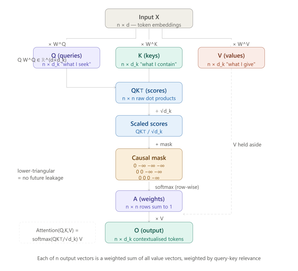
The first step of self-attention is to project each token’s embedding into three separate representations using learned weight matrices:$$Q = XW^Q, \quad K = XW^K, \quad V = XW^V$$where $W^Q, W^K, W^V \in \mathbb{R}^{d \times d_k}$​ are learned projection matrices, and $d_k$​ is the dimension of the query and key space (typically $d_k = d / h$ where $h$ is the number of attention heads, more on that shortly).

The resulting matrices $Q, K, V \in \mathbb{R}^{n \times d_k}$ are called the Query, Key, and Value matrices respectively.

The intuition behind this decomposition is often explained through an analogy: think of each token’s query vector as a question it is asking (“what context do I need?”), each token’s key vector as an advertisement of its content (“here is what I contain”), and each token’s value vector as the actual information it contributes when attended to (“here is what I give you if you attend to me”). The query-key interaction determines how much each token attends to every other; the values are what actually gets aggregated.

Scaled Dot-Product Attention

Given $Q$, $K$, and $V$, the attention output is computed as:$$\text{Attention}(Q, K, V) = \text{softmax}\!\left(\frac{QK^\top}{\sqrt{d_k}}\right) V$$Let’s unpack this step by step.

Step 1 — Dot products: $QK^\top \in \mathbb{R}^{n \times n}$ is a matrix of raw attention scores. Entry $(i, j)$ is the dot product between the query vector of token $i$ and the key vector of token $j$:$$s_{ij} = \mathbf{q}_i \cdot \mathbf{k}_j$$A high dot product means token $i$ finds token $j$ highly relevant. This is the mechanism through which, for example, a pronoun “she” can attend strongly to the noun “Alice” it refers to three sentences earlier.

Step 2 — Scaling: The dot products are divided by $\sqrt{d_k}$​​. Without this scaling, when $d_k$​ is large, the dot products grow large in magnitude, pushing the softmax into regions where gradients become vanishingly small — a variant of the vanishing gradient problem. The $\sqrt{d_k}$​​ factor keeps the variance of the dot products approximately constant regardless of model dimensionality.

Step 3 — Causal masking (decoder-only models): In autoregressive models like GPT, token $i$ must not attend to any token $j > i$ meaning that it cannot look into the future. Before applying softmax, a mask is added:$$s_{ij} \leftarrow s_{ij} + m_{ij}, \quad m_{ij} = \begin{cases} 0 & \text{if } j \leq i \\ -\infty & \text{if } j > i \end{cases}$$The $-\infty$ values become zero after softmax, effectively zeroing out future positions.

Step 4 — Softmax: Each row of the masked score matrix is passed through softmax:$$\alpha_{ij} = \frac{\exp(s_{ij})}{\sum_{k=1}^{n} \exp(s_{ik})}$$The resulting matrix $A \in \mathbb{R}^{n \times n}$ is the attention weight matrix. Each row sums to 1 and can be interpreted as a probability distribution over the sequence: the probability that token $i$ attends to each position.

Step 5 — Value aggregation: The output for token $i$ is a weighted sum of all value vectors:$$\mathbf{o}_i = \sum_{j=1}^{n} \alpha_{ij} \mathbf{v}_j$$In matrix form: $O = AV \in \mathbb{R}^{n \times d_k}$​. Each output vector is a contextualised representation of its token, so that the same word “bank” will produce a different output vector in “river bank” versus “central bank” because its attention weights will be distributed differently across the surrounding context.

Multi-Head Attention

A single attention head computes one set of query-key-value interactions. But different aspects of meaning may require different attention patterns simultaneously: a token might need to attend to its syntactic head, its semantic antecedent, and its positional neighbours all at once. Multi-head attention runs $h$ attention operations in parallel:$$\text{head}_i = \text{Attention}(QW_i^Q,\ KW_i^K,\ VW_i^V)$$ $$\text{MultiHead}(Q, K, V) = \text{Concat}(\text{head}_1, \ldots, \text{head}_h)W^O$$where $W_i^Q, W_i^K, W_i^V \in \mathbb{R}^{d \times d_k}$​ are per-head projection matrices, each head operates in a $d_k = d/h$ dimensional subspace, and $W^O \in \mathbb{R}^{d \times d}$ is a final output projection that mixes the concatenated heads back into the full $d$-dimensional space.

In GPT-3, $d = 12288$ and $h = 96$, so each head operates in a $d_k = 128$ dimensional subspace. The 96 heads learn to specialize: empirical work in mechanistic interpretability has identified heads that track syntactic subject-verb agreement, heads that copy tokens from earlier in context, heads that attend to the most recent noun phrase, and heads that implement induction — recognizing when a pattern seen earlier in the context is repeating.

The computational cost of full self-attention is $O(n^2 d)$, or quadratic in sequence length. For a 128K-token context window, the attention matrix alone has $128000^2 \approx 16$ billion entries, making naive computation prohibitively expensive. Efficient attention variants such as Flash Attention, Sparse Attention, Sliding Window Attention address this scaling problem, which we’ll cover in Part 3 alongside the full transformer block.

The KV Cache

During inference, a decoder-only model generates one token at a time. At step $t$, the model processes the full sequence $[t_1, \ldots, t_t]$ and predicts $t_{t+1}$​. Without optimization, this would require recomputing the key and value matrices for all previous tokens at every step so thar cost grows as $O(t^2)$ per generation.

The KV cache eliminates this redundancy. Since the key and value representations of tokens $t_1, \ldots, t_{t-1}$​do not change between steps (they depend only on those tokens’ positions and embeddings, which are fixed once generated), they can be cached in memory and reused. At step $t$, only the new token’s $Q$, $K$, $V$ need to be computed; the cached $K$ and $V$ matrices from previous steps are concatenated and the attention is computed against the full cached sequence.

This reduces per-step inference cost from $O(t^2)$ to $O(t)$ in attention computation, but at the cost of memory. A KV cache for a 128K-token context with 96 heads, 128 layers, and FP16 precision occupies on the order of tens of gigabytes. Managing KV cache memory is one of the primary challenges in deploying frontier models efficiently at scale. It is why inference hardware for long-context models requires far more VRAM than a naive parameter count would suggest.

What Attention Actually Learns

It is tempting to describe attention as a mechanism that “understands” language. It is more precise, and more useful for engineering purposes, to say that attention is a differentiable, content-based memory retrieval system. The model learns, through gradient descent on the next-token prediction objective, to configure its $W^Q$, $W^K$, $W^V$ matrices such that the right values get retrieved for the right queries.

The mechanism has no built-in notion of syntax, coreference, or meaning. All of that emerges from training dynamics or from the statistical regularities of billions of documents. Understanding this distinction is important for debugging model failures: when an LLM makes a coreference error or loses track of a constraint stated early in a long context, the failure mode is almost always traceable to attention weights that were distributed incorrectly, either because the training distribution underrepresented that pattern, or because the KV cache compression strategy discarded the relevant context.

Conclusion

Self-attention is the architectural innovation that made modern LLMs possible. By allowing every token to attend directly to every other token in a single parallelisable matrix operation, it solves the long-range dependency problem that defeated earlier sequential architectures. Multi-head attention extends this by learning multiple independent attention patterns simultaneously, while the KV cache makes autoregressive inference tractable at scale.

Part 3 will take the attention output $O \in \mathbb{R}^{n \times d}$ and trace it through the rest of the transformer block: the feed-forward network, layer normalisation, residual connections, and the architectural choices (decoder-only versus encoder-decoder) that distinguish GPT-style models from BERT-style ones.

Coming next in the AI Engineering series is Part 3: The Transformer Block and Architecture.