
-
How Large Language Models Work — Part 5: Inference, Sampling, Emergent Behaviour, and Open Frontiers
This is the final part of a five-part series on the internal mechanics of large language models. Parts 1–4 covered tokenization, embeddings, attention, the transformer block, and the training and alignment pipeline. Part 5 addresses inference: how a trained model generates text, the mathematics of sampling, context window management, emergent capabilities, and the open research frontiers shaping the next generation of LLMs.
From Trained Weights to Generated Text
A trained, aligned LLM is a fixed mathematical function: given a sequence of input tokens, it produces a probability distribution over the next token. Inference is the process of repeatedly applying this function to generate text, while the engineering decisions made at inference time have a surprisingly large impact on the quality, diversity, safety, and cost of model outputs.
At each generation step , the model computes:
where is the final-layer hidden state at position n, is the unembedding matrix (often tied to the transpose of the input embedding matrix WE), and the resulting vector of logits over vocabulary entries is passed through softmax to produce a probability distribution. A token is then drawn from this distribution (called the sampling step) appended to the context, and the process repeats.
The Mathematics of Sampling
How a token is selected from the output distribution is not trivial. Naive greedy decoding that always selects the highest-probability token tends to produce repetitive, degenerate outputs. Real systems use one or more of the following strategies.
Temperature scaling. Before applying softmax, the logits are divided by a temperature parameter T>0:
As , the distribution concentrates on the single highest-logit token, equivalent to greedy decoding. As , the distribution approaches uniformity with maximum entropy, maximum randomness. Values of are typical for creative generation; for precise factual or code generation tasks. Temperature does not change which token is most probable; instead, it changes how peaked or flat the distribution is.
Top-k sampling. The distribution is truncated to only the highest-probability tokens, which are then renormalised and sampled from. A typical value is . Top- prevents the model from sampling tokens with negligible probability, but it is sensitive to the shape of the distribution. In a uniform distribution, keeps 40 of many reasonable options; in a very peaked distribution, may retain tokens with near-zero probability.
**Nucleus (top-) sampling.** Rather than fixing the number of tokens, nucleus sampling fixes the cumulative probability mass: the smallest set of tokens such that is retained and renormalised. A typical value is or . Nucleus sampling adapts naturally to the distribution’s shape. A peaked distribution retains few tokens, a flat one retains many – this is now the dominant strategy in production systems.
Min-p sampling. A newer variant, increasingly adopted in open-source inference stacks, sets a dynamic minimum probability threshold relative to the top token: any token with is discarded. This keeps tokens that are meaningfully competitive with the best option while discarding genuinely improbable ones, and empirically reduces repetition more effectively than top-p at matched quality.
In practice, production inference systems combine multiple strategies: temperature scaling applied first to reshape the distribution, followed by top- or min- truncation, followed by top- as a hard ceiling. The specific combination and hyperparameters are treated as tunable properties of a deployment configuration, not fixed properties of the model itself.
Context Windows and Memory Management
Every inference call operates within a context window, which is the maximum sequence length the model can process in a single forward pass. For GPT-4, the context window is 128K tokens; for Gemini 1.5 Pro, it extended to 1 million tokens; Llama 3.1 supports 128K. Context window length is not a free parameter, rather, it is constrained by the quadratic attention cost and, critically, by KV cache memory.
As established in Part 2, the KV cache stores the key and value tensors for every previous token at every layer, avoiding redundant recomputation during autoregressive generation. The memory footprint is:
For a model with 96 layers, 96 heads, , processing a 128K-token context in FP16: GB. This exceeds the VRAM of any single current GPU by a factor of roughly 10, which is why long-context inference requires either model parallelism across multiple devices, quantisation of KV cache entries to lower precision (INT8 or INT4), or approximate attention methods that reduce what must be stored.
Several efficient attention variants address this scaling problem. Flash Attention (Dao et al., 2022) reorders the attention computation to avoid materialising the full attention matrix in high-bandwidth memory, reducing memory complexity from to while maintaining identical numerical output. Grouped-query attention (GQA), used in Llama 2 and 3, shares key and value heads across multiple query heads, reducing KV cache size by a factor of (the group size) without significant quality degradation. Sliding window attention, used in Mistral, restricts each token to attend only within a fixed window of recent tokens, allowing arbitrarily long sequences at the cost of cross-window recall.
Emergent Capabilities and Phase Transitions
One of the most scientifically consequential, and practically important, observations in LLM scaling is the phenomenon of emergent capabilities: abilities that are essentially absent in smaller models and appear abruptly as scale crosses some threshold, without being explicitly trained for.
Wei et al. (2022) documented dozens of such capabilities: few-shot chain-of-thought reasoning, multi-step arithmetic, word unscrambling, and logical deduction all exhibit sharp phase transitions: near-zero performance at sub-threshold scales, near-human performance above it. The sharpness of these transitions distinguishes emergence from smooth capability growth and has profound implications for predicting what a model trained at a given scale will be able to do.
The mechanism underlying emergence is debated. One influential account (the “grokking” hypothesis, from Power et al. at Anthropic) suggests that models first memorise training examples, then undergo a phase transition in which they discover a compressed algorithmic solution that generalises to held-out data. Another account, from Anthropic’s interpretability research, suggests that emergent capabilities correspond to the model assembling multi-step circuits, consisting of sequences of attention heads and FFN layers that compose to implement a non-trivial algorithm, and that these circuits can only form once the model has sufficient depth and width to represent all required intermediate computations simultaneously.
From an engineering standpoint, emergence creates a prediction problem. The GPT-3 scaling curve gave no warning that a GPT-4-scale model would exhibit chain-of-thought reasoning, code execution, or structured tool use. This motivates careful capability elicitation and evaluation at each new model generation —(the practice of red-teaming) as a safety and capability discovery discipline.
Chain-of-Thought and Reasoning Models
The most practically significant emergent capability is multi-step reasoning — and the discovery that it can be dramatically improved by prompting or training the model to externalise its intermediate steps.
Chain-of-thought prompting (Wei et al., 2022) established that providing examples of step-by-step reasoning in the prompt elicits dramatically better performance on multi-step arithmetic, commonsense reasoning, and symbolic manipulation tasks without any additional training. The effect is robust and scales with model size: smaller models gain little from chain-of-thought, but models above approximately 100B parameters show large, consistent improvements.
Reasoning models — exemplified by OpenAI’s o1 and o3, and Anthropic’s Claude’s extended thinking mode — take this further by training models to produce extended internal reasoning traces before generating a final answer. The training procedure uses reinforcement learning on verifiable outcomes: the model is rewarded for producing correct final answers to problems where correctness can be checked algorithmically (mathematics, code execution, formal logic), and the RL signal drives the model to develop longer, more structured reasoning traces that are instrumentally useful for producing correct outputs.
The result is a qualitatively different inference regime. A standard GPT-style model generates tokens in a single forward pass per token, with effective reasoning depth bounded by model depth. A reasoning model generates a long internal monologue, often thousands of tokens of scratchpad, before committing to an answer, effectively trading inference-time compute for reasoning quality. This represents a fundamental shift in the compute profile of AI: capability is no longer a fixed function of model size, but can be increased at inference time by allocating more tokens to reasoning.
Open Frontiers: Mechanistic Interpretability, Multimodality, and Agents
Three research frontiers are most likely to define the next phase of LLM development.
Mechanistic interpretability is the program of reverse-engineering what computations specific model components implement. The goal is to go beyond behavioural evaluation — what the model does — to structural understanding — what algorithm it uses to do it. Anthropic’s superposition hypothesis (Elhage et al., 2022) established that neural networks represent more features than they have dimensions by encoding features as directions in a high-dimensional space and tolerating controlled interference between them. The subsequent Sparse Autoencoder (SAE) program — also led at Anthropic — has made it possible to decompose model activations into sparse, interpretable features: human-understandable concepts that each activate for a specific, semantically coherent set of inputs. SAE-based interpretability tools are now being applied to frontier models at production scale, with the goal of identifying circuits responsible for deception, sycophancy, and unsafe behaviours before deployment.
Multimodality extends the transformer architecture beyond text. Vision-language models (GPT-4V, Gemini, Claude 3) process images by encoding them through a vision encoder — typically a Vision Transformer (ViT) — into a sequence of patch embeddings that are projected into the LLM’s token embedding space and concatenated with text tokens before the first transformer layer. Audio-language models (GPT-4o’s audio mode) follow an analogous pattern with a spectrogram encoder. The frontier is native multimodality — a single model trained end-to-end on text, image, audio, and video tokens simultaneously, rather than modality-specific encoders bolted onto a text backbone.
Agentic systems extend the inference loop beyond token generation to include tool use, memory retrieval, and sequential decision-making. An agent wraps an LLM in a loop: the model generates text that includes structured tool calls (web search, code execution, database queries); the tool results are appended to the context; the model continues generating, possibly issuing further tool calls, until it produces a final response. Multi-agent systems extend this further: multiple LLM instances, each with different system prompts and tool access, communicate with each other through structured message passing. The engineering challenges are significant — context management, tool reliability, error recovery, and safety alignment in agentic settings are all active areas of research — but the capability ceiling of agentic LLMs is substantially higher than single-turn generation.
A Map of the Whole
Across this five-part series, we have traced the complete path from raw string to generated output:
- Tokenization — BPE or SentencePiece converts text into integer token IDs from a vocabulary of 32K–256K entries.
- Embedding — each token ID is projected into a d-dimensional vector; positional information is added via learned embeddings, sinusoidal encoding, or RoPE.
- Attention — N transformer blocks each apply multi-head self-attention: Q, K, V projections; scaled dot products; causal masking; softmax; value aggregation.
- Feed-forward network — each block applies a position-wise two-layer MLP with SwiGLU activation, implementing key-value memory over learned factual associations.
- Training — next-token prediction loss over trillions of tokens; AdamW with cosine decay; Chinchilla-optimal compute allocation; distributed parallelism at scale.
- Alignment — SFT on human demonstrations, reward model training on preference rankings, RLHF with PPO or DPO to concentrate capability toward preferred outputs.
- Inference — temperature scaling, nucleus or min-p sampling, KV cache management, and extended chain-of-thought reasoning to generate high-quality outputs efficiently.
The transformer is a simple, composable architectural primitive. What it does, when trained at sufficient scale on sufficient data, and aligned to human preferences, is not simple at all.
This concludes the five-part series on how large language models work. If you have found this series useful, the natural next steps are the mechanistic interpretability literature (Anthropic’s Transformer Circuits thread), the Chinchilla and scaling laws papers, and Neel Nanda’s open-source interpretability tooling at TransformerLens.
-
How Large Language Models Work — Part 4: Training, Scaling Laws, and RLHF
This is Part 4 of a five-part series on the internal mechanics of large language models. Part 3 covered the complete transformer block and architectural variants. Part 4 addresses how models are trained: the pre-training objective, loss functions, the Chinchilla scaling laws, and the alignment pipeline of instruction tuning and RLHF that transforms a raw language model into a useful assistant.
The Pre-Training Objective
The entire capability of a modern LLM emerges from one deceptively simple training objective: predict the next token. Given a sequence of tokens , the model is trained to maximise the log-probability of each token given all preceding tokens:
This is the negative log-likelihood loss, or equivalently, cross-entropy between the model’s predicted distribution and the one-hot true distribution over the vocabulary. Minimising is equivalent to maximising the likelihood of the training corpus under the model.
The reason this objective is so productive is that predicting the next token accurately requires solving an enormous range of implicit sub-problems. To predict the next word in a chemistry paper, the model must understand chemistry. To predict dialogue in a novel, it must model character motivation and narrative consistency. To predict the output of a code snippet, it must simulate execution. All of these capabilities emerge as instrumental sub-goals of the single next-token prediction objective, a phenomenon sometimes called the “bitter lesson” of AI: simple objectives applied at scale consistently outperform hand-crafted inductive biases.
The training corpus for frontier models is correspondingly vast. GPT-3 was trained on roughly 300 billion tokens drawn from Common Crawl, WebText2, Books, and Wikipedia. Llama 3 used over 15 trillion tokens. Assembling, filtering, deduplicating, and quality-scoring a corpus at this scale is itself a major engineering undertaking, and corpus quality is widely understood to be among the most important determinants of downstream model capability, arguably more important than architectural choices at equivalent parameter counts.
The Training Loop
Pre-training proceeds through the standard deep learning training loop, applied at extreme scale:
Forward pass: A batch of token sequences is sampled from the corpus. Each sequence is processed through the full transformer stack consisting of embedding, N transformer blocks, and unembedding. This produces a probability distribution over the vocabulary at each position.
Loss computation: Cross-entropy loss is computed by comparing the model’s predicted distribution at each position with the true next token.
Backward pass: Gradients of the loss with respect to all θ parameters are computed via backpropagation through the entire network.
Parameter update: An optimiser, called Adam or AdamW in virtually all modern LLMs, applies the gradient update:
where and are bias-corrected first and second moment estimates of the gradient, and is the learning rate. AdamW adds a decoupled weight decay term directly to the parameter update, separate from the gradient. This is important because standard L2 regularisation interacts badly with Adam’s adaptive scaling, while decoupled weight decay does not.
The learning rate schedule typically involves a linear warmup phase (to avoid instability at the start of training when gradients are large and parameters are random) followed by a cosine decay to a minimum learning rate of roughly :
where is the total number of training steps. The cosine schedule has become the near-universal choice because it empirically outperforms linear decay and step schedules across model sizes and tasks.
At frontier scale, training runs on clusters of thousands of GPUs or TPUs, employing a combination of data parallelism (each device processes a different batch, gradients are aggregated), tensor parallelism (each layer’s weight matrices are sharded across devices), and pipeline parallelism (different layers run on different devices simultaneously). GPT-3’s training required approximately 3.14 × 10²³ FLOPs and ran on 10,000 V100 GPUs. A GPT-4-class training run is estimated at well over 10²⁵ FLOPs.
Scaling Laws and the Chinchilla Result
How should a fixed compute budget be allocated between model size (number of parameters ) and training data (number of tokens )? This is the central question addressed by neural scaling law research.
Kaplan et al. (OpenAI, 2020) established that loss scales as a power law in both and , and derived the now-famous result that, for a fixed compute budget , loss is minimised by scaling and in a roughly fixed ratio, with growing considerably faster than . This led to the prevailing practice of training very large models on relatively modest amounts of data, exemplified by GPT-3 (175B parameters, 300B tokens).
Hoffmann et al. (DeepMind, 2022) in the “Chinchilla” paper challenged this conclusion. Using a broader range of model sizes and more careful experimental design, they derived a different optimal allocation:
That is, compute-optimal training requires scaling parameters and tokens in a roughly 1:1 ratio. Their finding: for a given compute budget, the optimal model size is significantly smaller than previously believed, but must be trained on significantly more data. The compute-optimal ratio is approximately 20 training tokens per parameter.
The practical implication was dramatic. GPT-3, by the Chinchilla analysis, was massively undertrained. A 175B parameter model should be trained on approximately 3.5 trillion tokens to be compute-optimal, not 300 billion. Chinchilla itself (70B parameters, 1.4 trillion tokens) outperformed Gopher (280B parameters) on nearly every benchmark despite using a quarter of the parameters, simply by training longer on more data.
The Chinchilla result reshaped subsequent model development: Llama 1 and 2 trained smaller models on far more tokens; Llama 3 trained an 8B model on 15 trillion tokens. The scaling law itself takes the form:
where is the irreducible entropy of the data distribution (a lower bound on achievable loss), and , , , are empirically fitted constants. The three terms represent, respectively: the noise floor of the task, the contribution of model capacity, and the contribution of data quantity.
From Language Model to Assistant: Instruction Tuning and RLHF
A model trained only on next-token prediction is not a useful assistant. It will complete any prompt in the style of its training distribution and it might respond to “How do I bake bread?” by generating more questions rather than an answer, because question-continuation is a common pattern in web text. Transforming a base language model into a helpful, honest, and harmless assistant requires a second training phase: alignment.
The alignment pipeline used by OpenAI, Anthropic, Google DeepMind, and most frontier labs follows a three-stage process.
Stage 1 — Supervised fine-tuning (SFT): Human annotators write demonstrations of ideal assistant behaviour through prompt-response pairs that exhibit the desired properties: helpfulness, accuracy, appropriate refusal of harmful requests, appropriate tone and format. The base model is then fine-tuned on this dataset using standard cross-entropy loss. SFT alone substantially improves instruction-following; InstructGPT’s SFT model already significantly outperformed the raw GPT-3 base in human evaluations.
Stage 2 — Reward model training: Human annotators rank multiple model responses to the same prompt, from best to worst. A separate reward model , itself a transformer, is trained to predict these rankings. Given a prompt and response , the reward model produces a scalar score . The training objective minimises a pairwise ranking loss:
where is the preferred response, is the less preferred response, and is the sigmoid function. This Bradley-Terry loss encourages the reward model to assign higher scores to preferred completions.
Stage 3 — Reinforcement learning from human feedback (RLHF): The SFT model is further fine-tuned using the reward model as a proxy for human preference. The policy gradient objective maximises expected reward while penalising deviation from the SFT model via a KL divergence constraint:
The KL penalty, weighted by coefficient , is critical. Without it, the policy would rapidly overfit to the reward model’s blind spots, a phenomenon called reward hacking: the model learns to produce outputs that score highly according to while being nonsensical or subtly harmful in ways the reward model did not penalise. The KL term keeps the aligned model close to the original SFT distribution, preserving its language modelling capabilities while steering it toward preferred outputs.
This optimisation problem is solved using the Proximal Policy Optimisation (PPO) algorithm, which clips the policy gradient update to prevent excessively large steps. PPO is not the only approach; Direct Preference Optimisation (DPO), introduced in 2023, reformulates the RLHF objective as a supervised learning problem that bypasses the reward model entirely:
DPO has become widely adopted because it is significantly simpler to implement and more stable to train than PPO-based RLHF, while achieving comparable alignment quality on most benchmarks.
Why InstructGPT Outperformed GPT-3
The RLHF result that most concisely captures the importance of alignment is this: InstructGPT (1.3B parameters, RLHF-trained) was preferred by human evaluators over GPT-3 (175B parameters, base model) 85% of the time. A model with 100× fewer parameters that is aligned to human preferences consistently produced more useful outputs than its massive unaligned ancestor.
This result makes precise what “alignment” means in practice. A base model has vast latent capability distributed across its weights, but no particular disposition to deploy that capability in ways that are useful or safe. Alignment is the process of concentrating and directing that capability toward the response distribution humans actually want, without catastrophically degrading the underlying language modelling capability that makes the responses coherent.
Conclusion
Pre-training on next-token prediction, at compute-optimal scale guided by Chinchilla’s laws, produces a powerful but raw language model. The alignment pipeline (SFT → reward model → RLHF or DPO) shapes that raw capability into something useful, honest, and controllable. The gap between these two stages is where most of the practical engineering work in deploying frontier models resides.
Part 5 will close the series with inference: sampling strategies, the mechanics of context window management, emergent capabilities and what they imply, and the open research frontiers such as mechanistic interpretability, reasoning models, and multimodality. These will define the next phase of LLM development.
Part 5: Inference, Sampling, and Emergent Behaviour — the final instalment of this series.
-
How Large Language Models Work — Part 3: The Transformer Block and Architecture
This is Part 3 of a five-part series on the internal mechanics of large language models. Part 2 derived scaled dot-product attention and the KV cache. Part 3 traces the complete transformer block consisting of feed-forward networks, layer normalisation, and residual streams; it examines the architectural differences between decoder-only and encoder-decoder models.
From Attention Output to Transformer Block
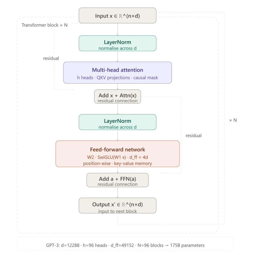
At the end of Part 2, self-attention had produced an output matrix or one updated vector per token, now containing contextual information drawn from every other position in the sequence. But this is only the first half of a single transformer block. Before the signal moves to the next layer, it passes through three more components: a residual connection, layer normalisation, and a position-wise feed-forward network. Together with multi-head attention, these four elements constitute the repeating unit of every transformer-based LLM, stacked times to form the full model.
Understanding each component precisely is important not just for implementation, but for diagnosing failure modes, interpreting mechanistic interpretability research, and making informed decisions about architectural variants when selecting or fine-tuning models.
Residual Connections
The residual connection, introduced in ResNets for computer vision and adopted into transformers from the outset, is deceptively simple. Rather than passing the attention output directly to the next component, the original input is added back:
This addition of the residual or skip connection has several important consequences.
First, it solves the vanishing gradient problem for very deep networks. During backpropagation, gradients flow backward through the network. Without residual connections, multiplying many Jacobians together through N sequential non-linear transformations causes gradient magnitudes to decay exponentially, making early layers extremely slow to learn. The residual path provides a direct gradient highway that bypasses each block, so that gradients can flow backward through the addition operation unchanged, regardless of how many layers separate the loss from the input.
Second, and more subtly, residual connections give the network an inductive bias toward learning incremental transformations. Rather than learning to reconstruct the full representation from scratch at each layer, each block learns only the delta or the correction to add to the existing representation. In mechanistic interpretability, researchers conceptualise the transformer as a residual stream: a -dimensional vector that is progressively written to and read from by successive attention heads and feed-forward layers, each contributing small structured updates. This framing, developed extensively by Anthropic, EleutherAI, and Neel Nanda’s research group, has proven highly productive for understanding what specific components of large models actually compute.
Layer Normalisation
Before and/or after each sub-component, layer normalisation is applied. For a vector :
where is the mean, is the standard deviation, is a small constant for numerical stability, and are learned scale and shift parameters.
Layer normalisation stabilises training by preventing the internal covariate shift problem, which is the tendency for the distribution of a layer’s inputs to change as upstream parameters update, forcing each layer to continuously readapt. By normalising each token’s representation independently across the feature dimension (as opposed to batch normalisation, which normalises across the batch dimension), layer norm is compatible with variable-length sequences and works correctly with batch size 1, making it well-suited for autoregressive inference.
Two conventions exist for where layer norm is placed within the block:
Post-norm (original Transformer, “Attention Is All You Need”): LayerNorm is applied after the residual addition:
Pre-norm (GPT-2, GPT-3, most modern LLMs): LayerNorm is applied to the input before the sub-component:
Pre-norm has become the dominant convention because it produces more stable training dynamics at large scale. Gradients flow more cleanly through the unmodified residual path, and the model is less sensitive to initialisation and learning rate choice. The architectural difference is subtle but has meaningful empirical consequences; models trained with post-norm often require careful learning rate warmup schedules that pre-norm models do not.
The Feed-Forward Network
After the attention sub-layer (with its own residual connection and layer norm), each transformer block applies a position-wise feed-forward network (FFN). The term “position-wise” means the same two-layer MLP is applied independently to each token’s vector, and the FFN has no cross-token interactions, unlike attention.
The standard formulation:
where , , and is the intermediate dimension, typically . In GPT-3, and , giving each FFN roughly million parameters, more than the attention sub-layer at that layer.
The activation function σ has evolved across generations. The original transformer used ReLU. GPT-2 and GPT-3 used GeLU (Gaussian Error Linear Unit), which approximates ReLU with a smooth, non-zero gradient for slightly negative inputs:
where is the standard normal CDF. More recent models use SwiGLU, a gated variant introduced by Noam Shazeer in 2020 and adopted in PaLM, Llama, and most frontier models:
where is the Sigmoid Linear Unit and is an additional learned gate projection. SwiGLU consistently outperforms GeLU on downstream benchmarks, though the underlying reason remains an active area of research. When using SwiGLU, is typically set to rather than to keep parameter counts comparable across architectures.
What does the FFN actually learn? Mechanistic interpretability work, particularly from Anthropic and the Neel Nanda group, has provided strong evidence that FFN layers function as key-value memories. Each row of acts as a pattern detector (a “key”), and the corresponding row of stores an associated “value” that gets added to the residual stream when that pattern is detected. This explains why larger FFNs improve factual recall (they have more memory slots) and why deleting specific FFN neurons can surgically remove specific factual associations from a model’s behaviour.
The Complete Transformer Block
Assembling all components, the full pre-norm transformer block for a decoder-only model is:
This two-step computation, attention followed by FFN, each with its own pre-norm and residual, is repeated times. In GPT-3, . In Llama 3 70B, . In a typical GPT-4-class model, is believed to be in the range of 96–120 layers. Each repetition allows the model to build increasingly abstract representations. Early layers handle low-level syntactic patterns, while later layers encode semantic and factual content.
Decoder-Only vs Encoder-Decoder Architecture
Two principal transformer architectures are in widespread use, differing in how they process input and generate output.
Decoder-only models (GPT, Llama, Mistral, Gemma, Falcon) use a single stack of transformer blocks with causal (masked) self-attention. Every token can attend only to previous tokens. The entire input prompt and the generated output share the same context window and are processed by the same stack. At inference time, the model autoregressively generates one token at a time, each conditioned on all prior tokens. This architecture is dominant for general-purpose language models because it scales efficiently and the training objective of next-token prediction across the entire sequence is simple, scalable, and empirically powerful.
Encoder-decoder models (T5, BART, mT5, the original Transformer for machine translation) use two distinct stacks. The encoder processes the full input with bidirectional attention. Every token can attend to every other token simultaneously, with no causal mask. The encoded representation is then passed to the decoder via a cross-attention mechanism: each decoder token’s query attends to the encoder’s key-value pairs in addition to previously generated decoder tokens. The cross-attention block takes the form:
This architecture was originally designed for sequence-to-sequence tasks such as translation, summarisation, or question answering, where the full input is available before generation begins. It has largely been supplanted by decoder-only models for general language tasks, primarily because the instruction-tuned decoder-only paradigm proved more flexible and scalable. However, encoder-decoder models retain advantages for tasks requiring deep understanding of a fixed input, such as structured prediction, constrained generation, and certain retrieval tasks.
A hybrid, the encoder-only model (BERT, RoBERTa, DeBERTa), uses bidirectional attention with no autoregressive generation. It is optimised for discriminative tasks such as classification, named entity recognition, or semantic similarity, rather than generation, and remains widely used in production embedding pipelines and retrieval systems.
Depth, Width, and the Scaling Hypothesis
The transformer block’s design raises a natural question: does it matter whether a model has more layers (depth) or larger hidden dimension (width)? Empirically, the two interact in complex ways, and the optimal allocation of a fixed parameter budget between depth and width is one of the central questions addressed by scaling law research, which is the subject of Part 4.
What is clear from both theory and experiment is that depth and width serve different functions. Width increases the model’s representational capacity at each layer by the size of the residual stream and the richness of the key-value memory in the FFN. Depth increases the number of sequential computational steps the model can take, which means the number of times attention and FFN transformations can be composed. Tasks requiring multi-step reasoning appear to benefit disproportionately from depth, while factual recall scales more uniformly with total parameter count regardless of how it is distributed between depth and width.
Conclusion
The transformer block is elegant in its modularity: a residual stream, two sub-components (attention and FFN), and two layer normalisation steps. The full model is simply this block repeated times. But the interactions between these components, including the gradient flow through residual connections, the factual storage in FFN key-value memories, and the progressive abstraction through depth, give rise to capabilities that are not predictable from any single component in isolation.
Part 4 will move from architecture to training: the next-token prediction objective, loss functions, the Chinchilla scaling laws, and the dramatic effect of RLHF and instruction tuning on model behaviour, explaining why InstructGPT, at a fraction of GPT-3’s parameter count, consistently outperformed it.
Coming next in the AI Engineering series is Part 4: Training, Scaling Laws, and RLHF.
-
How Large Language Models Work — Part 2: The Attention Mechanism
This is Part 2 of a five-part series on the internal mechanics of large language models. Part 1 covered tokenization, embeddings, and positional encoding. Part 2 derives the self-attention mechanism from first principles, covers multi-head attention, and examines the KV cache.
The Problem Attention Solves
At the end of Part 1, we had a matrix , which was a one d-dimensional vector per token, encoding both semantic identity and position. The first transformer layer receives this matrix and must do something critical: allow each token to incorporate information from every other token in the sequence before passing its updated representation to the feed-forward network.
This is the problem that self-attention solves. Earlier sequence models such as LSTMs and GRUs processed tokens sequentially, which meant that a word at position 1 had to wait for its influence to propagate through every intermediate hidden state to reach position 512. Long-range dependencies were difficult to learn because the gradient had to flow through hundreds of recurrent steps. Attention eliminates this bottleneck entirely by allowing any token to attend directly to any other token in a single operation, regardless of distance.
Queries, Keys, and Values
The first step of self-attention is to project each token’s embedding into three separate representations using learned weight matrices:where are learned projection matrices, and is the dimension of the query and key space (typically where is the number of attention heads, more on that shortly).
The resulting matrices are called the Query, Key, and Value matrices respectively.
The intuition behind this decomposition is often explained through an analogy: think of each token’s query vector as a question it is asking (“what context do I need?”), each token’s key vector as an advertisement of its content (“here is what I contain”), and each token’s value vector as the actual information it contributes when attended to (“here is what I give you if you attend to me”). The query-key interaction determines how much each token attends to every other; the values are what actually gets aggregated.
Scaled Dot-Product Attention
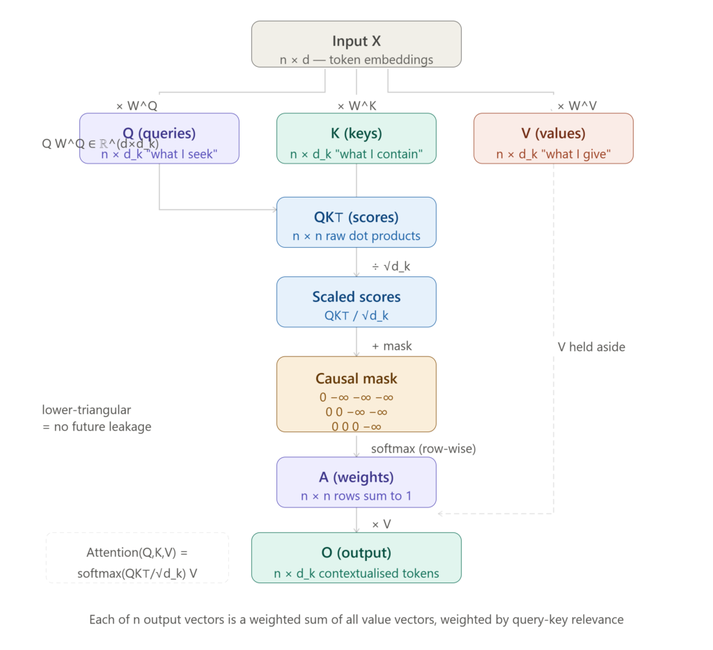
Given , , and , the attention output is computed as:Let’s unpack this step by step.
Step 1 — Dot products: is a matrix of raw attention scores. Entry is the dot product between the query vector of token and the key vector of token :A high dot product means token finds token highly relevant. This is the mechanism through which, for example, a pronoun “she” can attend strongly to the noun “Alice” it refers to three sentences earlier.
Step 2 — Scaling: The dot products are divided by . Without this scaling, when is large, the dot products grow large in magnitude, pushing the softmax into regions where gradients become vanishingly small — a variant of the vanishing gradient problem. The factor keeps the variance of the dot products approximately constant regardless of model dimensionality.
Step 3 — Causal masking (decoder-only models): In autoregressive models like GPT, token must not attend to any token meaning that it cannot look into the future. Before applying softmax, a mask is added:The values become zero after softmax, effectively zeroing out future positions.
Step 4 — Softmax: Each row of the masked score matrix is passed through softmax:The resulting matrix is the attention weight matrix. Each row sums to 1 and can be interpreted as a probability distribution over the sequence: the probability that token attends to each position.
Step 5 — Value aggregation: The output for token is a weighted sum of all value vectors:In matrix form: . Each output vector is a contextualised representation of its token, so that the same word “bank” will produce a different output vector in “river bank” versus “central bank” because its attention weights will be distributed differently across the surrounding context.
Multi-Head Attention
A single attention head computes one set of query-key-value interactions. But different aspects of meaning may require different attention patterns simultaneously: a token might need to attend to its syntactic head, its semantic antecedent, and its positional neighbours all at once. Multi-head attention runs attention operations in parallel: where are per-head projection matrices, each head operates in a dimensional subspace, and is a final output projection that mixes the concatenated heads back into the full -dimensional space.
In GPT-3, and , so each head operates in a dimensional subspace. The 96 heads learn to specialize: empirical work in mechanistic interpretability has identified heads that track syntactic subject-verb agreement, heads that copy tokens from earlier in context, heads that attend to the most recent noun phrase, and heads that implement induction — recognizing when a pattern seen earlier in the context is repeating.
The computational cost of full self-attention is , or quadratic in sequence length. For a 128K-token context window, the attention matrix alone has billion entries, making naive computation prohibitively expensive. Efficient attention variants such as Flash Attention, Sparse Attention, Sliding Window Attention address this scaling problem, which we’ll cover in Part 3 alongside the full transformer block.
The KV Cache
During inference, a decoder-only model generates one token at a time. At step , the model processes the full sequence and predicts . Without optimization, this would require recomputing the key and value matrices for all previous tokens at every step so thar cost grows as per generation.
The KV cache eliminates this redundancy. Since the key and value representations of tokens do not change between steps (they depend only on those tokens’ positions and embeddings, which are fixed once generated), they can be cached in memory and reused. At step , only the new token’s , , need to be computed; the cached and matrices from previous steps are concatenated and the attention is computed against the full cached sequence.
This reduces per-step inference cost from to in attention computation, but at the cost of memory. A KV cache for a 128K-token context with 96 heads, 128 layers, and FP16 precision occupies on the order of tens of gigabytes. Managing KV cache memory is one of the primary challenges in deploying frontier models efficiently at scale. It is why inference hardware for long-context models requires far more VRAM than a naive parameter count would suggest.
What Attention Actually Learns
It is tempting to describe attention as a mechanism that “understands” language. It is more precise, and more useful for engineering purposes, to say that attention is a differentiable, content-based memory retrieval system. The model learns, through gradient descent on the next-token prediction objective, to configure its , , matrices such that the right values get retrieved for the right queries.
The mechanism has no built-in notion of syntax, coreference, or meaning. All of that emerges from training dynamics or from the statistical regularities of billions of documents. Understanding this distinction is important for debugging model failures: when an LLM makes a coreference error or loses track of a constraint stated early in a long context, the failure mode is almost always traceable to attention weights that were distributed incorrectly, either because the training distribution underrepresented that pattern, or because the KV cache compression strategy discarded the relevant context.
Conclusion
Self-attention is the architectural innovation that made modern LLMs possible. By allowing every token to attend directly to every other token in a single parallelisable matrix operation, it solves the long-range dependency problem that defeated earlier sequential architectures. Multi-head attention extends this by learning multiple independent attention patterns simultaneously, while the KV cache makes autoregressive inference tractable at scale.
Part 3 will take the attention output and trace it through the rest of the transformer block: the feed-forward network, layer normalisation, residual connections, and the architectural choices (decoder-only versus encoder-decoder) that distinguish GPT-style models from BERT-style ones.
Coming next in the AI Engineering series is Part 3: The Transformer Block and Architecture.
-
How Large Language Models Work — Part 1: Tokenization and Embeddings
This is Part 1 of a five-part deep-dive series on the internal mechanics of large language models. This series is written for engineers, ML practitioners, and technically advanced readers. Part 1 covers tokenization and embeddings — the first two stages through which raw text becomes a mathematical object a neural network can reason over.
Why Text Must Be Transformed
Neural networks are, at their core, mathematical functions that operate on tensors, which are multi-dimensional arrays of floating-point numbers. They cannot accept raw text strings as input. Before a language model can do anything useful, it must convert a sequence of characters into a sequence of numbers. This two-step process of tokenization followed by embedding is where all LLM processing begins, and understanding it deeply is prerequisite to understanding everything that follows.
Stage 1: Tokenization
What a Tokenizer Does
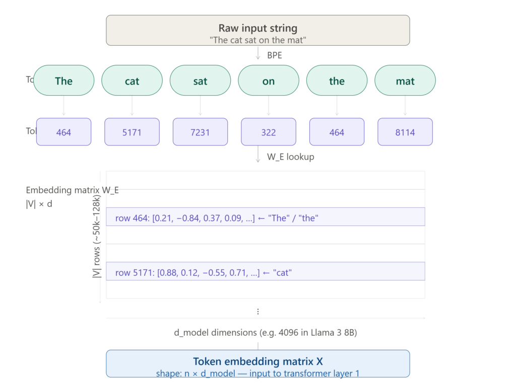
A tokenizer breaks a raw string into a sequence of discrete units called tokens, and maps each token to an integer index in a fixed vocabulary. Given the input string:
"The cat sat on the mat"a tokenizer might produce the token sequence: [464, 5171, 7231, 322, 464, 8114]
Each integer is an index into a vocabulary table of size , typically between 32,000 and 100,000 entries for modern models. GPT-4 uses a vocabulary of approximately 100,277 tokens. Llama 3 uses 128,256.
Byte-Pair Encoding (BPE)
The dominant tokenization algorithm used in modern LLMs is Byte-Pair Encoding (BPE), originally a data compression algorithm adapted for NLP by Sennrich et al. in 2016.
BPE builds its vocabulary through an iterative merging process:
- Initialise the vocabulary with every individual character (or byte) in the training corpus.
- Count all adjacent symbol pairs across the corpus.
- Merge the most frequent pair into a single new symbol.
- Repeat steps 2–3 until the vocabulary reaches the target size ∣V∣.
The result is a vocabulary that contains individual characters, common subwords, and frequent whole words. The word “tokenization” might be represented as three tokens:
token,izationis further split intoiz,ationdepending on training corpus frequency.This has a critical practical consequence: no word is ever truly unknown to a BPE tokenizer. Any string, including code, URLs, foreign scripts, or novel proper nouns, can be decomposed into its constituent bytes if nothing else matches. This is why BPE-based models generalise to inputs they have never seen verbatim.
Token Fertility and Efficiency
Not all languages tokenize equally efficiently. English text typically tokenizes at roughly 0.75 tokens per word. Languages with richer morphology, such as Finnish, Turkish, Arabic, or non-Latin scripts, tokenize less efficiently, sometimes requiring 3–5 tokens per word. This has practical implications: a context window of 128,000 tokens holds far more English prose than it does Thai or Arabic text, a bias baked into the model’s architecture from the vocabulary construction stage.
The fertility of a tokenizer, or the average number of tokens per word, is a meaningful measure of how well it serves a given language or domain. Code-optimised models like DeepSeek Coder use vocabularies with explicit code tokens to reduce the fertility of common programming constructs.
WordPiece and SentencePiece
Two notable alternatives to BPE are worth knowing:
WordPiece, used in BERT and its derivatives, is similar to BPE but merges pairs that maximise the likelihood of the training data under a language model, rather than simply the most frequent pair. This produces slightly different vocabulary distributions.
SentencePiece, used in models including Llama and T5, treats the input as a raw unicode byte stream with no pre-tokenization step (no whitespace splitting). This makes it language-agnostic and particularly well-suited for multilingual models.
Stage 2: Token Embeddings
The Embedding Matrix
Once tokenization has produced a sequence of integer indices , each index must be converted into a dense vector. This is done via an embedding matrix , where is the model’s hidden dimension (also called the embedding dimension or ).
The embedding for token ti is simply a row lookup:In GPT-3, . In Llama 3 8B, . This single matrix, learned entirely from data during pre-training, is responsible for encoding the semantic relationships between all tokens in the vocabulary.
The number of parameters in the embedding matrix alone is . For GPT-4’s approximate configuration, that is which is often hundreds of millions of parameters just for this one component.
Why Dense Vectors Work: The Geometry of Meaning
The remarkable property of learned embeddings is that semantic relationships emerge as geometric relationships in . The classic demonstration is the linear analogy:
This is not programmed. It emerges from the statistical structure of co-occurrence patterns in the training corpus. Words that appear in similar contexts end up with similar embedding vectors, measured by cosine similarity:In high-dimensional spaces, this geometry becomes extraordinarily rich. Directions in embedding space can encode syntactic roles, semantic fields, sentiment polarities, and factual associations — all simultaneously, in different orthogonal subspaces of the same .
Stage 3: Positional Encoding
Token embeddings encode what each token is, but they contain no information about where in the sequence each token appears. The sequence
"dog bites man"and"man bites dog"would produce identical sets of token embeddings in a different order and would be catastrophic for a model that needs to understand syntax and word order.Positional information must therefore be injected explicitly.
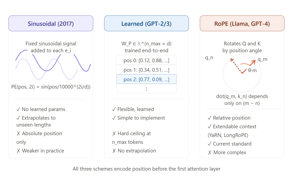
Sinusoidal Positional Encoding (Original Transformer)
The original transformer paper (Vaswani et al., 2017) proposed adding a fixed sinusoidal signal to each token embedding. For position pos and dimension i:
The input to the first transformer layer is then:
The sinusoidal formulation has a useful property: the positional encoding of position can be expressed as a linear function of the encoding at pos, which makes it easy for attention heads to learn to attend to tokens at a fixed relative offset.
Learned Positional Embeddings
GPT-2 and GPT-3 replaced sinusoidal encodings with learned positional embeddings: a second matrix , where is the maximum context length. Position pos adds the row to the token embedding. These are learned end-to-end during pre-training and tend to slightly outperform sinusoidal encodings on benchmarks, at the cost of a hard context length ceiling — the model cannot generalise beyond positions it has seen during training.
Rotary Positional Embedding (RoPE)
The current state of the art for most frontier models, including Llama, Mistral, GPT-4, and Gemini, is Rotary Positional Embedding (RoPE), introduced by Su et al. in 2021.
Rather than adding a positional vector to the token embedding, RoPE encodes position by rotating the Query and Key vectors in the attention mechanism (covered in Part 2) by a position-dependent angle. For a vector at position m in dimension pair :
where .
The critical advantage: the dot product between a query at position m and a key at position n depends only on their relative offset , not their absolute positions. This gives the model a natural inductive bias toward relative position awareness, and with extensions like YaRN makes it possible to extend the effective context window well beyond what the model was trained on.
RoPE is why modern models can be fine-tuned to handle 128K or even 1M token context windows without retraining the entire model from scratch.
Putting It Together: The Input Representation
The final input to the first transformer layer for a sequence of n tokens is a matrix :where is the positional encoding for position (sinusoidal, learned, or RoPE-derived). Each row of is a -dimensional vector carrying both the semantic identity of the token and its position in the sequence. This matrix is what flows into the self-attention mechanism, which is the subject of Part 2.
Key Numbers to Anchor Your Intuition
Model Vocabulary Positional scheme GPT-2 50,257 768–1,600 Learned GPT-3 50,257 12,288 Learned Llama 3 8B 128,256 4,096 RoPE Mistral 7B 32,000 4,096 RoPE Gemma 2 256,000 2,304–3,584 RoPE
Conclusion
Before a single attention head fires, a large language model has already done substantial mathematical work. A raw string has been segmented into subword tokens by a BPE or SentencePiece algorithm, each token has been projected into a high-dimensional vector space where geometry encodes meaning, and position information has been woven in either additively or, in modern models, rotationally via RoPE. The quality of this input representation has an outsized effect on everything downstream: models with poorly constructed vocabularies or weak embedding initialisations are harder to train and less capable at convergence.
Part 2 will take this matrix and walk through exactly what the self-attention mechanism does with it, including the full mathematical derivation of scaled dot-product attention, multi-head attention, and what different heads actually learn to represent.
Coming next in the AI Engineering series is Part 2: The Attention Mechanism.
-
A History of Artificial Intelligence — Part 3: From Transformers to ChatGPT — and What It Means for the Strong AI Debate
This is the final part of a three-part series on the history of AI. Part 1 covered AI’s philosophical origins and the Turing Test, Strong AI vs. Weak AI, and Searle’s Chinese Room argument. Part 2 traced the rise of machine learning and deep learning through the founding of OpenAI in 2015. Part 3 picks up the story with the breakthrough that made ChatGPT possible.
The Paper That Changed Everything
By 2017, deep learning had already transformed computer vision and game-playing AI, as Part 2 described. But language remained stubbornly difficult. Earlier neural network architectures processed text sequentially, word by word, which made them slow to train and bad at capturing relationships between distant words in a sentence.
In June 2017, a team of researchers from Google Brain and Google Research published “Attention Is All You Need,” introducing the Transformer architecture. The paper demonstrated that an architecture using only attention mechanisms, with no recurrence or convolutions at all, could outperform existing approaches on machine translation while training significantly faster.
The key innovation was self-attention. Self-attention allows each word, or token, in a sequence to attend to every other token in that same sequence, enabling efficient parallelization and much better modeling of long-range relationships between words. Because the architecture could process entire sequences of text at once rather than one word at a time, it enabled the training of dramatically larger and more sophisticated models than had previously been practical.
Few people, including the paper’s own authors, anticipated just how far-reaching this idea would become. Within a few years, researchers had adapted the Transformer architecture to tasks far beyond language translation, including image classification, image generation, and even protein folding.
GPT-1 to GPT-3: Teaching Machines to Predict the Next Word
The original 2017 Transformer had two halves: an encoder for reading text and a decoder for generating it. OpenAI was the first to apply generative pre-training specifically to the decoder half of this architecture, introducing the GPT-1 model in 2018. While other researchers, such as the team behind Google’s BERT, pursued clever training objectives, OpenAI took a more deceptively simple path: training models to predict the next word in a sequence, an approach now called language modeling. GPT pioneered the idea of pre-training language models on vast amounts of unlabeled text before fine-tuning them on specific downstream tasks.
The first GPT model had 117 million parameters and meaningfully advanced state-of-the-art results across many language tasks, but it was not GPT-2, with its 1.5 billion parameters, that began capturing genuine public attention. Each generation scaled up dramatically. GPT-2 followed in February 2019, and GPT-3 arrived in June 2020 with 175 billion parameters, demonstrating striking emergent capabilities that simply hadn’t been visible in smaller models. GPT-3 was the first model OpenAI commercialized broadly, through a private beta of the OpenAI API in June 2020. Meaning that for the first time, developers anywhere could build applications on top of a frontier language model without training one themselves.
But GPT-3, for all its scale, had a problem: it was powerful but not particularly easy to work with. Interacting with raw GPT-3 could be hit-or-miss; the model sometimes gave irrelevant answers or followed instructions only loosely. It was capable, but not especially helpful or safe by default.
Teaching the Model to Listen: RLHF and InstructGPT
The solution OpenAI developed would prove just as important as the scaling breakthroughs that preceded it: Reinforcement Learning from Human Feedback, or RLHF. The technique worked in stages: human AI trainers had conversations with the model and provided examples of good responses; the model then generated multiple possible answers to the same questions; human reviewers ranked these answers from best to worst; and the model learned to produce responses more like the highly ranked ones. arxiv
This fine-tuning stage, layered on top of GPT-3’s existing pre-training, became known as reinforcement learning with human feedback. OpenAI released the resulting model, InstructGPT, in early 2022, and the results were striking: human evaluators preferred InstructGPT’s outputs over raw GPT-3’s outputs 85% of the time, even though InstructGPT used far fewer parameters. That finding reframed the entire scaling debate: a smaller, better-aligned model could outperform a larger, unaligned one on the metrics that actually mattered to users.
RLHF didn’t just make models safer; it made them more useful in practical settings, because their responses became more predictable, more direct, and less prone to drifting into irrelevant territory.
November 30, 2022: ChatGPT Arrives
This period of refinement directly produced ChatGPT, which applied RLHF to a GPT-3.5 base model and packaged it inside a simple, conversational interface. OpenAI released ChatGPT on November 30, 2022, as a free research preview.
The public response was immediate and unprecedented. Within five days of launch, ChatGPT reached one million users, and an estimated 100 million monthly users within roughly two months, making it the fastest-adopted consumer product in history at that time.
What made ChatGPT spread so quickly wasn’t necessarily a leap in raw capability over what came before. The technical capabilities of InstructGPT and ChatGPT were almost identical — the primary changes OpenAI made were adding conversational training data and further tuning the training process. What changed was accessibility: for the first time, a frontier AI model was wrapped in an interface anyone could use, for free, with no technical knowledge required. The gap between “powerful research model” and “tool my grandmother can use” had finally closed.
From there, the pace of iteration accelerated further. GPT-4 arrived in March 2023 with image input and substantially stronger reasoning, followed by GPT-4 Turbo, then GPT-4o in May 2024, which combined text, audio, and image processing into a single model. A parallel “reasoning” lineage (the o-series, beginning with o1 in 2024) introduced models trained to work through an internal chain of thought before answering, particularly strengthening performance on math, coding, and science tasks. ChatGPT itself evolved from a simple chat box into a far broader platform capable of browsing, file analysis, and increasingly autonomous task execution.
Returning to the Question We Started With
This brings us back to where Part 1 began: Turing’s question of whether machines can think, and Searle’s challenge to the idea that they ever truly could.
Modern language models like ChatGPT are, at their technical core, exactly the kind of system Searle’s Chinese Room argument was built to describe: a process that manipulates symbols or tokens according to learned statistical patterns, without any claimed inner experience of meaning. Searle’s argument was never meant to deny that such a machine could produce remarkably intelligent-seeming behavior; it was aimed specifically at the philosophical claim that symbol manipulation alone is sufficient to produce genuine understanding. By that standard, today’s most advanced chatbots remain, in the strictest philosophical sense, firmly in weak AI territory. They are extraordinarily capable simulators of conversation, whatever may or may not be happening “underneath.”
Even ChatGPT itself is best understood as an advanced form of narrow AI, rather than a step toward the kind of general intelligence imagined at Dartmouth in 1956. It cannot reason about domains outside its training in the way a human professional moves fluidly between unrelated fields of expertise. It does not possess goals, desires, or self-awareness in any sense most philosophers would recognize as minds typically do.
And yet, six decades after Turing’s original 1950 paper, the Turing Test feels almost quaint. Millions of people now hold conversations daily with systems that, for stretches at a time, are functionally indistinguishable from a knowledgeable human correspondent. The technical bar Turing imagined has, in many everyday contexts, been cleared, even as the philosophical question he set out to sidestep remains as unresolved as ever.
What today’s AI does prove, decisively, is something Turing himself anticipated: that behavior, not metaphysics, is what changes the world. Whether or not ChatGPT “understands” anything in Searle’s sense, it has already reshaped how hundreds of millions of people write, code, research, and learn. The history traced across these three articles, from Turing’s question, through symbolic AI and its winters, through the rise of neural networks and deep learning, to the Transformer and RLHF, is ultimately the story of a field that kept building useful tools, even while the deepest question that started it all remains open.
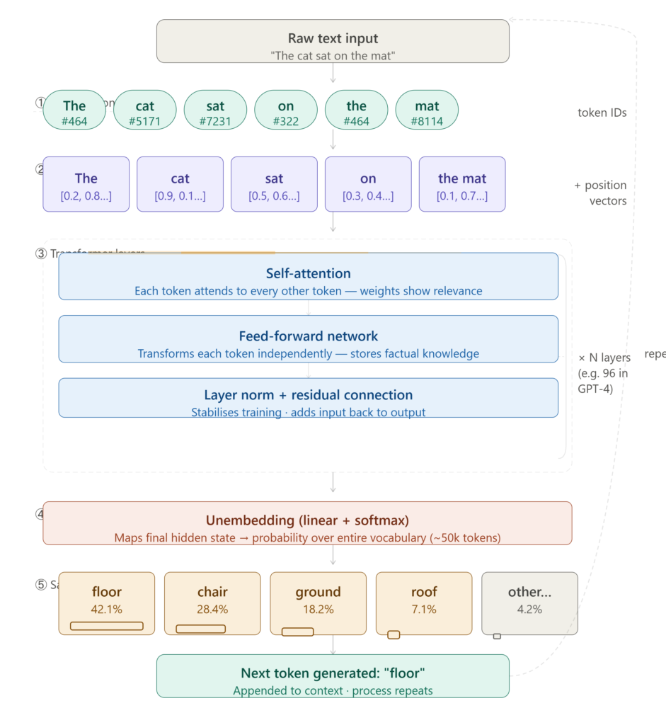
Here’s the full end-to-end LLM pipeline in one diagram. It walks through five stages:
① Tokenization — raw text is split into token IDs (shown as pills with their vocabulary numbers).
② Embedding — each token ID is converted to a high-dimensional vector, plus a positional vector so the model knows word order.
③ Transformer layers — the heart of the model: self-attention (where each token “looks at” every other token, with amber lines showing attention weights from “sat”), a feed-forward network per token, and layer normalisation — repeated N times (96 layers in GPT-4).
④ Output projection — the final hidden state is mapped back across the entire vocabulary using a softmax to produce probabilities.
⑤ Sampling — a token is selected from the distribution (here “floor” wins at 42.1%), appended to the context, and the whole process repeats — shown by the dashed feedback arrow on the right.
This concludes our three-part series on the history of artificial intelligence. Explore more in our AI Foundations category, including beginner-friendly guides to AI tools, prompt engineering, and AI productivity.
-
A History of Artificial Intelligence — Part 2: The Machine Learning Revolution and the Road to OpenAI
This is Part 2 of a three-part series tracing the history of artificial intelligence. Part 1 covered AI’s philosophical origins, the Dartmouth Conference, and the AI winters. Part 2 picks up with the shift toward machine learning and traces the path to the founding of OpenAI.
A New Approach: Learning From Data Instead of Rules
By the end of Part 1, AI research had hit a wall. The symbolic, rule-based approaches of expert systems, sometimes retroactively called “Good Old Fashioned AI”, involved pre-programming knowledge and rules directly into a system. These approaches were brittle and difficult to scale. A quieter alternative had existed since the field’s earliest days but had never become mainstream: machine learning.
In machine learning, instead of a human programmer writing the rules, the program learns the rules itself from data. Arthur Samuel coined the term “machine learning” itself and was the first to apply the technique, building a self-learning checkers program in 1959 that ran on IBM mainframes. The idea was decades ahead of the computing power needed to make it practical.
The foundational building block for this approach was the artificial neural network, loosely inspired by the structure of the brain. An early version, the Perceptron, was a simple neuron-like model that learned to classify inputs. A 1969 analysis by Minsky and Papert highlighted the perceptron’s limitations, triggering a temporary retreat from neural network research — one of the contributing causes of the AI winters discussed in Part 1.
Backpropagation: The Algorithm That Made Deep Learning Possible
The technique that would eventually revive neural networks was backpropagation. It was a method for training multi-layered networks by calculating how much each connection contributed to an error, then adjusting it accordingly. Backpropagation allowed multi-layer neural networks to adjust their weights to minimize errors, enabling these networks to automatically learn useful internal representations of data.
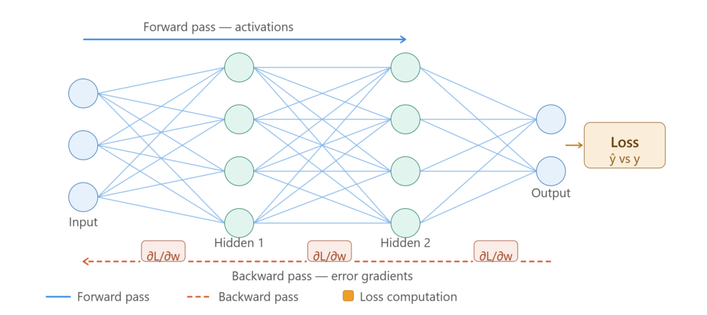
In the above diagram, the blue forward pass carries activations left to right through the input layer, two hidden layers, and the output layer, with all the inter-neuron weight connections visible. The amber loss box on the right computes the difference between the predicted output and the true label. The coral dashed backward pass then carries the error gradient right to left, and the
∂L/∂wpills mark the points at each layer boundary where weights get adjusted using the chain rule.In 1986, Geoffrey Hinton, David Rumelhart, and Ronald Williams developed and popularized backpropagation, making the training of multi-layered neural networks genuinely feasible for the first time. In 1989, Yann LeCun provided one of the first practical demonstrations of the technique at Bell Labs, combining convolutional neural networks with backpropagation to read handwritten digits, a system that would later be used to process handwritten numbers on bank checks.
The timing was bittersweet. This breakthrough arrived just as the second AI winter (roughly 1985 to the early 1990s) was setting in, as overly optimistic claims about AI’s “immediate” potential had broken expectations and angered investors, pushing the phrase “artificial intelligence” toward something close to pseudoscience status in some circles. Backpropagation’s true potential would have to wait.
The 1990s: Quiet Progress Beneath the Surface
Even during the chill of the AI winter, important work continued. Throughout the 1990s, Yann LeCun pioneered convolutional neural networks (CNNs), laying the technical foundation for modern computer vision. This is the technology that today powers everything from photo tagging to facial recognition. Researchers also developed the support vector machine, an effective system for mapping and classifying similar data, broadening the machine learning toolkit beyond neural networks alone.
The decade also delivered AI’s first major public spectacle. In 1997, Deep Blue, a chess program built at IBM, defeated reigning world chess champion Garry Kasparov, relying not on deep learning but on brute-force search combined with expert-crafted evaluation rules. It captured global headlines and reignited public fascination with AI, even though the underlying technology was closer to the symbolic AI of earlier decades than to the neural approaches that would soon take over.
The Data Explosion and the ImageNet Moment
Two ingredients were still missing for deep learning to fulfill its promise: enough data to learn from, and enough computing power to process it. The internet supplied the first. The internet boom of the 1990s and 2000s provided machine learning systems with vast quantities of real-world data to learn from for the first time.
Recognizing this, Stanford professor Fei-Fei Li began building ImageNet in 2006, an enormous database that would eventually contain more than 14 million labeled images, designed specifically to give machine learning systems the structured data they needed to learn effectively. Li summarized the philosophy behind the project simply: data drives learning.
Computing power, the second missing ingredient, arrived through an unlikely source: graphics processing units (GPUs), originally built for video games. By 2011, GPU speeds had increased significantly enough to train convolutional neural networks without the cumbersome layer-by-layer pre-training that had previously been necessary.
These two trends collided in 2012, in what is widely considered the single most important turning point in modern AI history. AlexNet, developed by Alex Krizhevsky, Ilya Sutskever, and Geoffrey Hinton, won the ImageNet competition, and its success demonstrated that deep learning had decisive advantages in both efficiency and accuracy over older approaches, sparking the deep learning revolution that defines the current era of AI. The rapid adoption of this feature-learning approach by major technology companies followed almost immediately.
From Vision to Strategy: Deep Learning Spreads
Once deep learning proved itself on image recognition, it rapidly expanded into other domains. In 2014, Ian Goodfellow and colleagues introduced Generative Adversarial Networks (GANs), a technique that enabled AI systems to generate convincingly realistic data, an early ancestor of today’s AI image generators.
Perhaps the most striking demonstration of deep learning’s power came from the world of board games. Unlike older symbolic chess programs that relied on pre-programmed evaluation functions, Google DeepMind’s AlphaGo combined deep learning with Monte Carlo tree search, using a neural network to evaluate which moves were promising rather than relying purely on brute-force calculation. In 2015, AlphaGo defeated the world champion Go player, a feat many AI researchers had assumed was still decades away, since Go’s branching complexity vastly exceeds that of chess. AlphaGo achieved this by playing millions of simulated games against itself, learning optimal strategies through deep reinforcement learning rather than human-programmed rules.
2015: The Founding of OpenAI
It was against this backdrop of accelerating breakthroughs and growing public and academic concern about where increasingly powerful AI systems might lead that a new kind of organization was born. In 2015, Elon Musk, Sam Altman, Greg Brockman, and other co-founders established OpenAI, with an explicit mission to promote safe and open AI development.
The founding represented something distinct from the corporate AI labs that had driven progress up to that point. Rather than developing AI purely as a commercial product, OpenAI was structured around the idea that increasingly powerful AI systems needed an organization explicitly focused on ensuring their benefits were broadly shared, and their risks carefully managed. At the time, few could have predicted just how central this organization would become to the AI story over the following decade.
The stage was now set. Deep learning, massive datasets, GPU computing, reinforcement learning, and several other tools, were all in place. What remained was a breakthrough in how machines processed language itself, one that would lead directly to the creation of the Generative Pre-trained Transformer, and eventually, to ChatGPT.
This is Part 2 of a 3-part series on the history of AI. Part 3 will trace the development of the Transformer architecture, the GPT model family, and the creation of ChatGPT — closing the loop on the strong AI vs. weak AI debate raised in Part 1.
-
A History of Artificial Intelligence — Part 1: From Ancient Dreams to the Birth of a Field
This is Part 1 of a three-part series tracing the history of artificial intelligence, from its philosophical roots to the creation of OpenAI and ChatGPT. Part 1 covers the early foundations of AI through the AI winters of the 1970s and 80s.
Before the Machines: A Question, Not a Technology
Long before computers existed, humans imagined artificial beings capable of thought — from mechanical automatons in ancient myth to philosophical debates about the nature of mind. But the scientific story of AI begins not with a machine, but with a question. In the 1950s, researchers started exploring whether intelligence could be formalized, tested, and eventually built into machines.
The foundations were laid even earlier than most people realise. In 1943, Warren McCulloch and Walter Pitts published a paper proposing the first mathematical model of a neural network, a concept that would lie mostly dormant for decades before becoming the backbone of modern deep learning. It is a useful reminder that AI’s history is rarely linear; many of its most important ideas were proposed long before the technology existed to realize them.
Alan Turing and the Question “Can Machines Think?”
Alan Turing, often considered the father of modern computing, made many important contributions to artificial intelligence. In 1950, he published his landmark paper “Computing Machinery and Intelligence,” introducing what would later be known as the Turing Test.
Rather than getting tangled in unanswerable philosophical debates about consciousness, Turing proposed something practical: if a machine could convincingly communicate like a human in conversation, its intelligence should be taken seriously. In his proposed experiment, a human evaluator interacts with both a human and a machine without knowing which is which; if the evaluator cannot reliably distinguish between them, the machine is said to have passed the test.
This was a deliberately pragmatic move. It set the tone for decades of AI research: intelligence would be measured by what a system could do, not by philosophical claims about what was happening inside it. That framing of behavior over inner experience would later become the central fault line in one of AI’s most enduring philosophical debates, which we’ll return to shortly.
1956: The Dartmouth Conference and the Birth of a Field
In the summer of 1956, a small group of researchers gathered at Dartmouth College for a workshop proposed by John McCarthy, Marvin Minsky, Nathaniel Rochester, and Claude Shannon. Their proposal stated the conjecture plainly: that every aspect of learning or any other feature of intelligence could in principle be so precisely described that a machine could be made to simulate it.
It was McCarthy’s coinage of “artificial intelligence” that appeared in that proposal, and the phrase stuck partly because the alternatives on offer were worse: “machine intelligence” was vague, and “cybernetics” was already associated with control theory rather than cognition. The workshop was loosely organized and not everyone stayed the full two months, but it established the field’s founding ambition: to simulate, in a machine, every aspect of human intelligence.
Remarkably, one team arrived with a working demonstration already in hand. Allen Newell and Herbert Simon, working with programmer Cliff Shaw, had built the Logic Theorist, a program designed to prove theorems from Whitehead and Russell’s Principia Mathematica. It successfully proved 38 of the first 52 theorems, and one of its proofs was, according to its creators, more elegant than the original. This is widely considered the first true AI program.
The momentum continued quickly. In 1958, John McCarthy developed the Lisp programming language, which became a primary tool for AI research for decades. In 1966, Joseph Weizenbaum created ELIZA, an early natural language program that simulated conversation and famously convinced some users they were talking to a sympathetic listener, despite running on simple pattern-matching rules.
Strong AI, Weak AI, and the Debate That Followed
As programs like ELIZA grew more convincing, a deeper question resurfaced: were these systems actually thinking, or just simulating the appearance of thought? This is the distinction between what philosophers call strong AI and weak AI.
Strong AI is the view that a suitably programmed computer can genuinely understand language and possess mental capabilities similar to a human’s and not merely simulate them. Weak AI, by contrast, holds that computers are useful tools for modeling or simulating mental processes, without making any claim that they actually understand or are truly intelligent.
This distinction became the center of one of the most famous thought experiments in the philosophy of AI: John Searle’s Chinese Room argument, published in 1980.
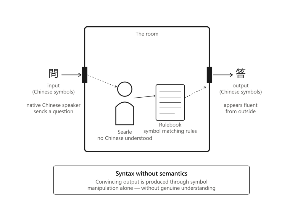
Searle asked readers to imagine a person who does not understand Chinese, sealed inside a room. This person is given Chinese characters through a slot in the door, along with a detailed rulebook (written in a language they do understand) for manipulating those symbols and producing appropriate Chinese characters in response. By following the rules precisely, the person can produce convincing Chinese replies (enough to pass a Turing Test) without ever understanding a single word of Chinese.
Searle’s point was that the person in the room and a computer running a program are not meaningfully different: both follow step-by-step instructions to produce outputs that appear intelligent, without any genuine understanding occurring. The argument was specifically directed at strong AI’s claim that an appropriately programmed computer, given the right inputs and outputs, would have a mind in exactly the same sense humans do. Searle aimed to show that information processing alone, no matter how sophisticated, cannot by itself produce genuine thought or understanding.
The argument was controversial and it remains so. One major line of response, known as the “Systems Reply,” concedes that the person inside the room doesn’t understand Chinese, but argues that some larger system: the room, the rulebook, and the person together might understand, even if no individual component does. A related “Virtual Mind” reply argues the real claim of strong AI isn’t that the computer itself understands, but that the process running on the computer creates a mind that understands, much like a character in a video game. Importantly, the Chinese Room argument was never meant as an attack on AI’s practical capabilities; it does not claim there is a limit to how intelligent a machine’s behavior can appear. Its target was narrower: the philosophical claim that computation alone is sufficient to produce genuine understanding.
Decades later, as language models like ChatGPT produce remarkably fluent conversation, Searle’s question has only grown more relevant, and we’ll return to it directly in Part 3 of this series.
The AI Winters: When Promises Outpaced Reality
The optimism of the 1950s and 60s could not last forever. The field experienced periods of decline known as “AI winters” in the 1970s and late 1980s, driven by unmet expectations and limited computational power. AI winters happened when expectations outpaced reality. Limitations in compute, data, and real-world performance made it difficult to deliver on the bold promises researchers had made, and funding agencies pulled back accordingly.
There was a partial revival before the deepest freeze set in. A resurgence in the 1980s was driven by the development of expert systems — programs that encoded the knowledge of human experts as explicit if-then rules, which found genuine commercial applications in narrow domains like medical diagnosis and chemical analysis. But even expert systems proved brittle and expensive to maintain at scale, and by the late 1980s, a second, harsher AI winter set in.
It would take a very different approach, one centered on learning from data rather than hand-coded rules, to pull the field out of its second winter and toward the breakthroughs that would eventually make modern AI possible. That story, including the rise of machine learning, deep learning, and the neural networks that power today’s chatbots, is where Part 2 picks up.
This is Part 1 of a 3-part series on the history of AI. Part 2 will cover the rise of machine learning and deep learning, leading up to the founding of OpenAI. Part 3 will trace the path from GPT to ChatGPT and discuss what these developments mean for the strong AI vs. weak AI debate today.
-
The Governance Imperative: Why Agentic AI Deployment Is Outpacing Enterprise Readiness
From Pilot Fatigue to Production Reality
Enterprise AI has crossed a threshold. Gartner forecasts that 40% of enterprise applications will embed task-specific AI agents by end of 2026, up from under 5% in 2025. That is not incremental adoption, it is a structural reconfiguration of how enterprises orchestrate work. The transition from isolated generative AI experiments to production-grade, multi-agent architectures is no longer a roadmap item. It is happening now, unevenly, and largely ahead of the governance frameworks designed to contain it.
The numbers are unambiguous about the asymmetry. Only 8% of organisations globally have a comprehensive AI governance framework, while 88% are actively using AI across business functions. That eighty-point gap is not a compliance footnote but the operating risk profile of most enterprises deploying agentic systems today.
The Governance Gap Is a Performance Variable, Not a Compliance Checkbox
Enterprise leaders who still frame AI governance as a risk management exercise are misreading the data. Companies using AI governance tools get over 12 times more AI projects into production. Organisations that use evaluation tools move nearly six times more AI systems to production. Governance, in other words, is the primary determinant of deployment velocity, not a constraint on it.
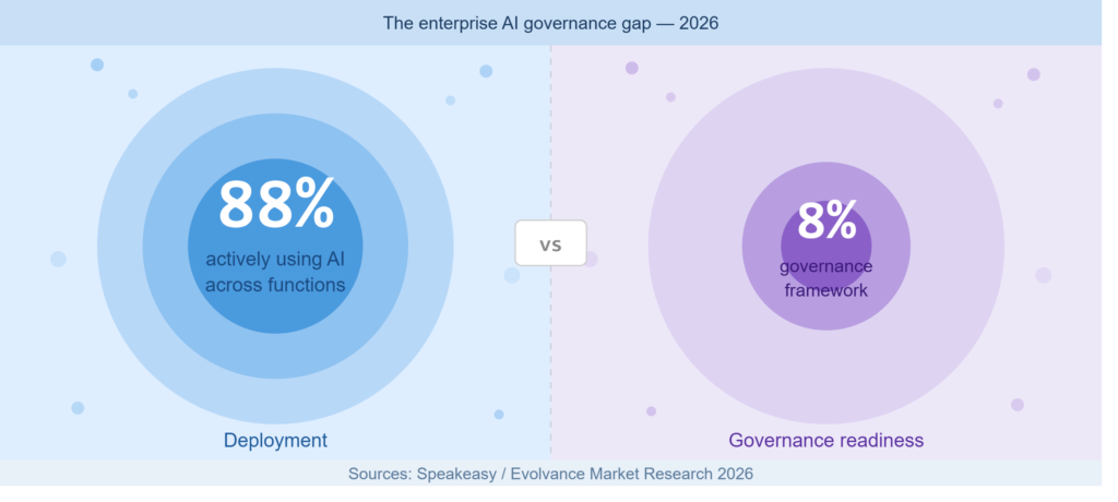
PwC research finds that 74% of all AI-generated economic value is captured by just 20% of organisations, and those AI leaders invest in governance infrastructure at rates significantly higher than the market average. The value concentration this represents is not coincidental. Mature governance programs eliminate the rework cycles, incident responses, and regulatory interventions that bleed velocity from under-governed programs.
The EU AI Act’s full enforcement provisions for high-risk AI systems take effect August 2, 2026, covering credit scoring, employment decisions, and insurance underwriting, with fines reaching €15 million or 3% of global annual turnover for non-compliance. For heavily regulated industries, this regulatory pressure compounds what is already an operational imperative.
Agentic Architecture Introduces an Entirely New Attack Surface
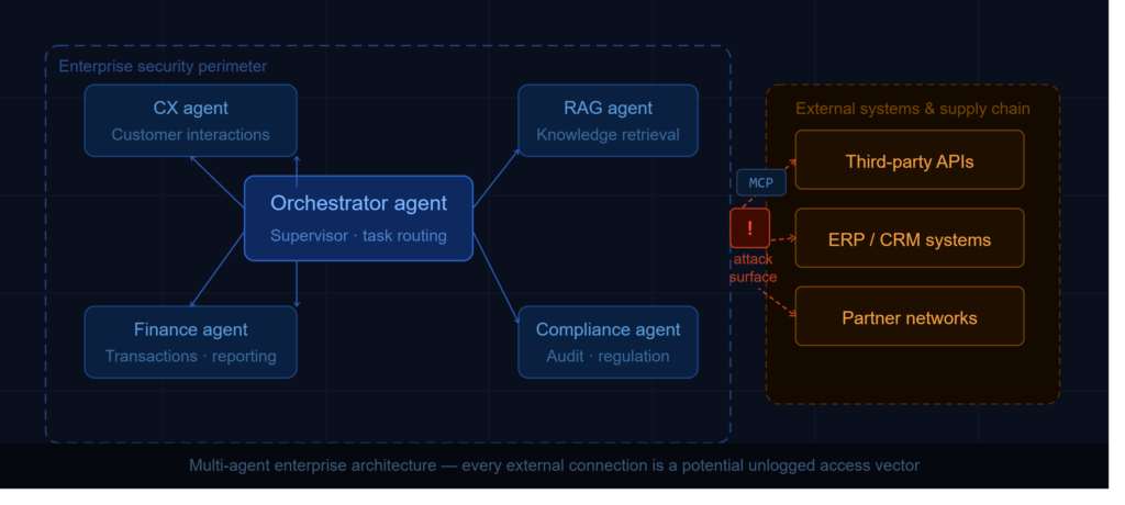
The shift to multi-agent systems does not merely scale existing risk. It introduces qualitatively new categories of it. Agents have identity, privileges, and access to systems and data across the business and out into the extended supply chain, either directly or through interfacing with other agents indirectly. This makes them a new and unexplored security risk, which is an entirely new non-deterministic attack surface.
The NSA released MCP security guidance in May 2026, signaling that federal regulatory requirements are a matter of when, not whether. The Model Context Protocol, which has rapidly matured into a common foundation for agent-to-tool connectivity, enables agents to interact with tools and data sources through standardised interfaces, a vital step toward portability, security, and observability. But standardisation alone does not constitute governance.
Uber’s deployment at scale offers the most instructive production case study available. By early 2026, 84% of Uber’s developers were using agentic coding tools daily, with AI generating between 65% and 72% of all code written inside their IDEs. Uber reached that scale because it built three governance layers before scaling adoption: an LLM gateway handling PII redaction, access control, and audit logging across every model interaction; an MCP gateway governing every agent-to-tool connection across 10,000+ internal services; and an agent identity system extending Zero Trust infrastructure to multi-agent workflows. The sequencing matters: governance infrastructure preceded scale, not the other way around.
Vendor Architecture Is a Strategic Decision, Not a Procurement Decision
Choosing an agentic AI vendor in 2026 is a different kind of decision. The model you select shapes how your agents reason, what they can and cannot do, how your data is handled, and how deeply you become entangled in a vendor’s ecosystem.
The compounding lock-in risk deserves particular attention. If agents run on a vendor’s proprietary orchestration layer, lock-in compounds at every layer of the stack. Enterprises that have not yet defined their agentic AI architecture strategy are already making a default choice. And that default is usually determined by whichever vendor has the best marketing rather than the best governance posture.
Sovereign AI considerations are now reshaping vendor selection in regulated industries. Sovereignty spans infrastructure, security, governance, lifecycle management, hiring policies, supply chains, service contracts, and partnerships, well beyond a one-time infrastructure decision. For European enterprises in particular, open-weight models with EU jurisdictional alignment offer a combination of flexibility and data sovereignty that hyperscaler-tied deployments cannot match.
What Separates Scaling Organisations from Those That Stall
Only 25% of AI initiatives deliver expected ROI, and only 16% reach enterprise-wide scale. Gartner expects over 40% of agentic AI projects to be cancelled by end of 2027 due to with escalating costs, unclear business value, and inadequate risk controls cited as primary drivers.
The distinguishing variable across the data is consistent: enterprises where senior leadership actively shapes AI governance achieve significantly greater business value than those delegating the work to technical teams alone. Governance, in the highest-performing organisations, is not a CISO concern or a legal review but a board-level operating discipline.
For enterprise AI leaders, the strategic question in the second half of 2026 is no longer whether to deploy agentic systems. It is whether the governance, evaluation, and observability infrastructure already in place is commensurate with the autonomy being granted. The organisations that answer that question honestly (and close the gap before scaling further) are precisely the ones that will capture the disproportionate share of value the data consistently points to.
-
When the AI Boom Meets Reality: Understanding the June 2026 Stock Selloff
A Turbulent Week for AI Stocks
The artificial intelligence sector has been one of the most exciting investment stories of the past several years. But in late June 2026, the mood shifted sharply. On June 23–24, 2026, the tech-heavy Nasdaq dropped 2.21% and the S&P 500 fell 1.44%, as investors sold semiconductor and AI-related shares broadly. The impact did not stay confined to Wall Street. South Korea’s Kospi index tumbled 10%, tripping a circuit breaker (an automatic 20-minute trading halt) with memory chipmakers SK Hynix and Samsung each falling more than 12%.
In total, semiconductor stocks shed more than $1.3 trillion in market value during this correction. For many observers, the question became urgent: is this the beginning of an AI bubble bursting, or simply a market pausing to catch its breath?
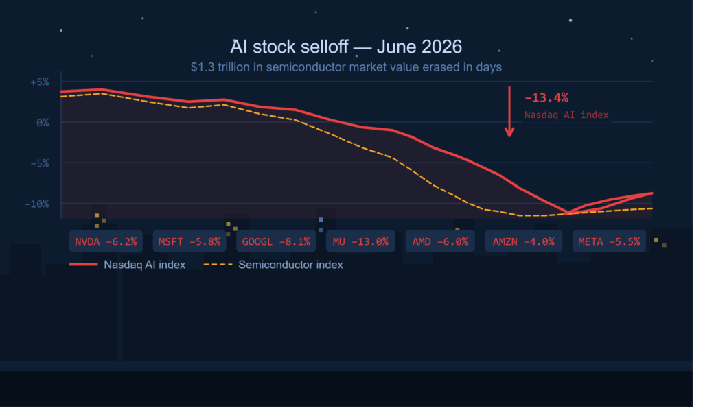
What Triggered the Selloff?
There was no single dramatic event that caused the drop. Instead, several slow-building pressures converged at once.
Spending without proof of returns. The most fundamental concern driving the selloff is a straightforward one. Combined 2026 capital expenditures across Microsoft, Alphabet, Amazon, and Meta exceeded $452 billion, while free cash flow at these companies declined dramatically. Investors who were once content to fund AI’s promise are now demanding evidence of profit. Goldman Sachs’s equity research head James Covello summarised the mood bluntly: “At some point, you’ve got to make money.” Enterprise surveys in 2025–2026 found that 95% of corporate AI projects delivered no measurable return.
Talent departures rattled confidence. High-profile AI talent departing from Google DeepMind to competitors, including Nobel Prize-winning researcher John Jumper to Anthropic, and Gemini co-lead Noam Shazeer to OpenAI. And these departures raised questions about competitive advantages, wiping $270 billion from Alphabet’s market cap.
Cautious guidance from chip companies. Broadcom’s Q3 AI chip sales guidance of $16 billion fell short of the $17.2 billion analyst estimate, and the company notably did not raise its full-year AI semiconductor forecast. This triggered a “sell-the-news” reaction, sending Broadcom shares down 14% and creating a ripple effect across the entire chip supply chain.
Valuation fatigue. AI stock valuations had been flying high for several years, built mainly on the technology’s promise rather than the bottom-line profit growth that fuels most companies’ stock price increases. After nine consecutive weeks of gains for the S&P 500, profit-taking was inevitable.
Correction, Not Collapse
It is important to keep this in perspective. Most analysts describe June 2026 as a correction rather than a crash. Tech earnings are still growing, and the Nasdaq remains up 10% for the year despite the selloff.
Micron Technology, the memory and storage chipmaker, surged nearly 16% after reporting stellar earnings, driven by the boom in demand for its semiconductors. That tells a more nuanced story: the underlying demand for AI infrastructure has not disappeared. What has changed is investors’ patience for returns on that investment.
Implications for the AI Industry
This market correction carries several important signals for anyone building in or investing around AI.
Monetisation is now the priority. The era of rewarding AI companies simply for spending boldly is ending. Businesses that can demonstrate clear, measurable returns from their AI investments will attract continued support. Those with vague AI strategies face sustained pressure.
Smaller and open-source models gain relevance. Some analysts argue that AI-related stock prices are falling in tandem with the cost of compute, as more companies question whether frontier models from OpenAI and Anthropic justify the premium when a reliable, lower-cost model may meet their needs perfectly well.
IPO timelines may shift. OpenAI is reportedly considering delaying its IPO because of recent market volatility, which could make it harder for the company to achieve its desired $1 trillion valuation.
Global ripple effects. When hyperscalers pour hundreds of billions into AI data centres, they compete for the same memory chips and components that consumer electronics also need, meaning the AI investment boom is one reason your next PC upgrade costs more than your last one.
What This Means for Learners and Builders
For students and professionals building skills in AI engineering, this correction is not a reason for concern; it is rather a reason to focus. Markets are not rejecting AI; they are demanding that AI deliver. That shift creates a clear opportunity for people who can build practical, results-driven AI solutions rather than theoretical demonstrations.
The companies and professionals who will thrive in the next phase of AI are those who can answer one question clearly: what problem does this solve, and how does it create measurable value? That question has always mattered. Now, the market is insisting on an answer.