The Science of AI
In-depth technical articles exploring the concepts behind artificial intelligence, including neural networks, machine learning algorithms, model architectures, and the mathematical foundations of AI.
-
How AI in Drug Discovery Is Critically Transforming Clinical Trials, Multi-Omics, and the Road Ahead — Part 3: Systems Biology, Patient Stratification, and Open Challenges
This is the final part of a three-part series on AI in drug discovery. Part 1 covered molecular representations, graph neural networks, and transfer learning for QSAR modelling. Part 2 covered protein structure prediction with AlphaFold, generative molecular design, and deep learning virtual screening. Part 3 examines how AI is being applied beyond the molecule: to systems-level disease biology, clinical trial optimisation, and the open theoretical and practical challenges that remain.
Beyond the Molecule
Parts 1 and 2 of this series focused on AI in drug discovery at the molecular scale: representing chemical structures, predicting binding affinities, generating candidate molecules, and screening compound libraries computationally. These approaches operate primarily on the drug-target interaction as an isolated system. But disease biology is not isolated. A drug candidate that binds its intended target with nanomolar affinity may fail in clinical trials because the disease it is meant to treat is driven by a complex network of interacting molecular processes, only one node of which is the chosen target.
The next frontier in AI in drug discovery is the integration of this systems-level complexity into the computational pipeline. This requires moving from molecular representations of individual compounds to multi-modal representations of biological systems: gene expression profiles, protein interaction networks, genomic variants, epigenetic modifications, metabolite concentrations, and clinical phenotypes, simultaneously. It also requires applying AI to the later stages of the pipeline where most drug failures actually occur: clinical trial design, patient stratification, and the prediction of clinical outcomes from pre-clinical data.
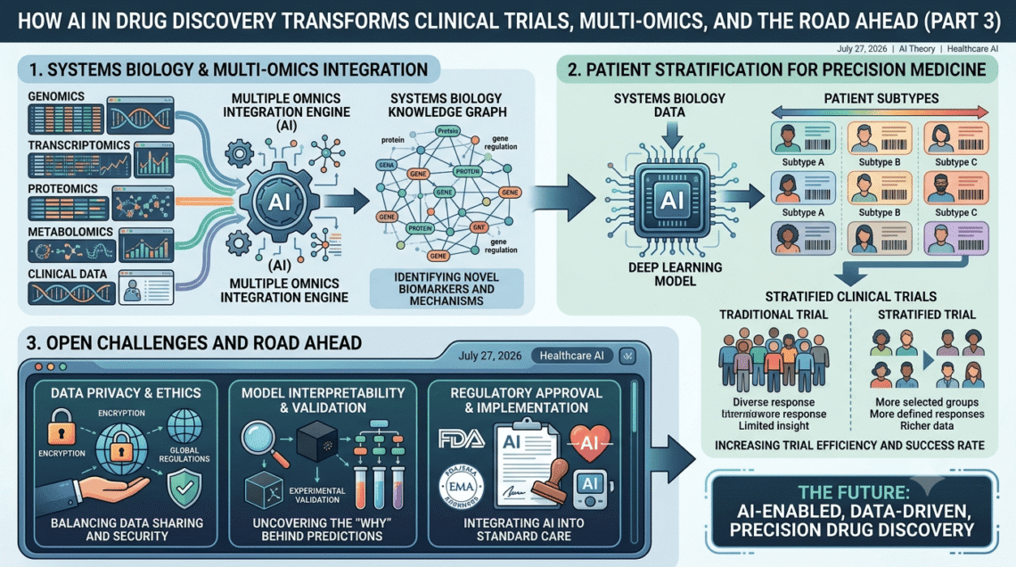
Multi-Omics Integration and Disease Biology
The term “omics” refers to the large-scale measurement of biological molecules at a systems level. Genomics measures DNA sequence variants. Transcriptomics measures gene expression levels across the genome. Proteomics measures protein abundances and modifications. Metabolomics measures the concentrations of small-molecule metabolites. Epigenomics measures chemical modifications to DNA and histones that regulate gene expression without changing the sequence. Each of these data modalities provides a partial view of the molecular state of a cell, tissue, or organism. Integrating them provides a far richer picture of disease biology than any single modality can offer.
Multi-omics data integration presents substantial machine learning challenges. The datasets are high-dimensional: a transcriptomics dataset may have expression measurements for 20,000 genes across thousands of patient samples. They are heterogeneous: different modalities have different scales, noise characteristics, and missing data patterns. They are multi-scale: genomic variants act through intermediate molecular mechanisms to produce phenotypic consequences, and causal relationships must be traced across these scales. And they are confounded: patient samples differ in age, sex, tissue type, disease stage, and treatment history in ways that must be accounted for before meaningful biological signals can be extracted.
The dominant deep learning approach for multi-omics integration is multi-modal representation learning. A separate encoder network is trained for each data modality, projecting high-dimensional omics measurements into a shared low-dimensional embedding space. The encoders are trained jointly using a contrastive objective that brings the embeddings of matched samples (different modalities measured from the same patient) close together while pushing the embeddings of unmatched samples apart:
where and are the embeddings of sample in modalities and , is cosine similarity, and is a temperature parameter. This objective, directly analogous to the CLIP contrastive loss used in vision-language models, produces a shared embedding space in which biological similarity is encoded as geometric proximity regardless of which combination of modalities was measured for a given sample.
The shared embeddings produced by multi-omics integration models have been used for disease subtype discovery, biomarker identification, and drug repurposing, finding new therapeutic applications for existing approved drugs. In the context of AI in drug discovery, multi-omics integration is most powerful when it is used to identify the molecular signatures that distinguish patients who respond to a drug from those who do not, which is the patient stratification problem at the heart of clinical trial design.
Knowledge Graphs and Biological Network Reasoning
A complementary approach to multi-omics integration for AI in drug discovery is the use of biological knowledge graphs: large heterogeneous graphs that encode known relationships between genes, proteins, diseases, drugs, pathways, and phenotypes, extracted from databases such as UniProt, DrugBank, DisGeNET, and the Gene Ontology. A node in a biological knowledge graph might represent a protein, a disease, a drug, or a biological pathway, and edges encode relationships such as “drug inhibits protein,” “gene is associated with disease,” or “protein participates in pathway.”
Graph neural networks applied to biological knowledge graphs can predict new edges: new drug-target interactions, new gene-disease associations, or new drug repurposing opportunities. The theoretical basis for these predictions is the relational inductive bias of graph neural networks: patterns of connectivity in the known graph carry information about the probability of unknown connections. A drug that inhibits several targets known to be involved in Alzheimer’s disease pathology is more likely to be therapeutically relevant to Alzheimer’s than a drug with no such connections, even if this association was never explicitly entered into the knowledge base.
Relational graph convolutional networks (R-GCNs) extend the message-passing framework of standard GNNs to heterogeneous graphs with multiple edge types. For a node v with neighbours of relation type r:
where is a relation-specific weight matrix, is the set of neighbours of under relation , and is a normalisation constant. This architecture allows the model to learn distinct aggregation functions for different biological relationship types, which is essential for reasoning over the heterogeneous entity types in a biological knowledge graph.
The knowledge graph approach to AI in drug discovery has produced notable results in drug repurposing. During the COVID-19 pandemic, knowledge graph models trained on pre-pandemic biological databases predicted several drug candidates that were subsequently validated in clinical studies, demonstrating that the relational information encoded in known biology carries genuine predictive signal for novel therapeutic questions.
Clinical Trial Optimisation and Patient Stratification
The majority of drug failures in AI in drug discovery occur not in the laboratory but in clinical trials, and the majority of those failures are attributable to efficacy failures rather than safety. A drug that works in the average patient population may fail in a heterogeneous trial cohort because the biological mechanism it targets is only active in a specific patient subgroup. Identifying that subgroup prospectively, before the trial begins, is the patient stratification problem.
AI approaches to patient stratification use the multi-omics representations described above to cluster patients by molecular subtype, identify biomarkers that predict treatment response, and design enriched trial cohorts that are more likely to show a statistically detectable treatment effect. The theoretical framework is that of heterogeneous treatment effect estimation: the goal is not to estimate the average treatment effect across the population but to estimate the conditional average treatment effect for each patient as a function of their molecular and clinical features:
where and are the potential outcomes under treatment and control respectively, and is the patient feature vector. Causal forest models and their neural network extensions, including the TARNet and DragonNet architectures, estimate from observational or randomised trial data while controlling for confounding between the patient features and treatment assignment.
Beyond patient stratification, AI in drug discovery is being applied to trial design itself. Bayesian adaptive trial designs use AI models to update the trial protocol in response to accumulating data, adjusting dose levels, sample sizes, and patient inclusion criteria based on interim results. Synthetic control arms, generated by matching trial patients to historical patient records using deep learning-based propensity models, can reduce the size of placebo arms and accelerate trial timelines. And natural language processing models applied to electronic health records can identify eligible patients for recruitment significantly faster than manual chart review, which is one of the principal bottlenecks in trial execution.
Foundation Models for Biology
The most significant recent development in AI in drug discovery is the emergence of large foundation models pre-trained on biological sequence data at a scale comparable to the language model pre-training described in the LLM series on this blog. ESM-3, released by EvolutionaryScale in 2024, is a 98-billion-parameter model jointly trained on protein sequences, structures, and functional annotations. Like a language model predicting the next token in a text sequence, ESM-3 learns to predict masked amino acid residues, masked structural tokens, and masked functional labels simultaneously, producing a unified representation of protein biology across sequence, structure, and function.
For AI in drug discovery, foundation models for biology offer the same advantages that LLM pre-training offers for natural language tasks: rich general-purpose representations that can be fine-tuned on small labelled datasets for specific prediction tasks, dramatically reducing the data requirements for new applications. A foundation model pre-trained on hundreds of millions of protein sequences and structures can be fine-tuned to predict the effect of a specific mutation on drug binding affinity using only a few hundred experimental measurements, a capability that classical QSAR methods could not approach at this sample size.
The logical extension of sequence-level foundation models is multi-modal biological foundation models that integrate molecular, cellular, tissue, and organismal data simultaneously. Projects including Geneformer, scGPT, and the Biological Foundation Model consortium are pursuing this vision, training transformer architectures on single-cell RNA sequencing data from tens of millions of cells to learn general-purpose cellular representations.
The theoretical aspiration of this line of research is a model that can answer arbitrary questions about biological systems: what is the effect of inhibiting this protein in this cell type in this disease context? This is the generalised inverse problem of systems biology, and it is the horizon toward which the most ambitious applications of AI in drug discovery are oriented.
Open Challenges and Theoretical Limitations
An honest assessment of AI in drug discovery requires acknowledging the substantial theoretical and practical challenges that remain, and that partially explain why the transformation of the drug development pipeline has been slower than the most optimistic early predictions suggested.
The data quality problem is perhaps the most fundamental. Machine learning models are only as good as their training data, and biological activity data is notoriously noisy, heterogeneous, and difficult to compare across experimental protocols. IC50 measurements, the most common metric of binding affinity in drug discovery datasets, can vary by an order of magnitude between laboratories for the same compound and target, depending on assay conditions, cell lines, and measurement protocols. Models trained on these heterogeneous datasets learn to fit the noise as well as the signal, producing predictions that generalise poorly to new experimental settings.
The distribution shift problem is closely related. Drug discovery models are trained on historical datasets of compounds that have been prioritised by human medicinal chemists using their own intuitions about what makes a good drug candidate. The training distribution is therefore heavily biased toward certain chemical scaffolds, certain target classes, and certain disease areas. Models trained on these datasets may perform well in regions of chemical space near the training distribution but fail catastrophically when applied to genuinely novel scaffolds or target classes. This is particularly concerning for AI in drug discovery, because the most valuable applications are precisely those that require exploring regions of chemical space far from what has been studied before.
The synthesis and experimental validation bottleneck constrains the practical impact of even the most accurate computational models. A generative model can propose millions of candidate molecules in hours, but each candidate must still be physically synthesised and experimentally tested before it can progress. Synthesis is slow, expensive, and frequently fails for complex or novel structures. The gap between computational proposal and experimental validation remains the primary rate-limiting step in AI in drug discovery pipelines, and closing it requires advances in automated synthesis and high-throughput experimental biology that are progressing but not yet at the scale that would fully exploit the computational capabilities described in this series.
The causal inference problem is perhaps the deepest theoretical challenge. Predicting that a molecule will bind to a target is a correlation problem. Predicting that inhibiting a target will produce a therapeutic benefit in patients is a causal problem. The distinction matters enormously: many targets that are statistically associated with disease in genomic studies turn out not to be causal drivers of disease, and drugs that inhibit them fail in clinical trials despite performing well in pre-clinical models.
AI models trained on correlational data cannot reliably distinguish causal from spurious associations without additional structure, either in the form of experimental interventional data (which is expensive) or causal modelling assumptions (which may not hold). Incorporating causal reasoning into AI in drug discovery is an active research frontier at the intersection of machine learning, statistics, and molecular biology.
Conclusion: What AI in Drug Discovery Can and Cannot Yet Do
AI in drug discovery has already produced tangible contributions at every stage of the pipeline this series has examined. AlphaFold has made protein structure prediction routine, enabling structure-based drug design for targets that were previously inaccessible. Deep learning scoring functions have accelerated virtual screening by orders of magnitude. Generative models are proposing molecules in previously unexplored regions of chemical space. Multi-omics integration is enabling patient stratification approaches that were not possible with classical biostatistics. And foundation models for biology are beginning to provide the kind of general-purpose biological reasoning that could eventually make the idealised version of AI-driven drug discovery a practical reality.
What AI in drug discovery cannot yet do is reliably translate these molecular-level capabilities into clinical success. The 90% clinical trial failure rate has not yet moved significantly, and the gap between pre-clinical AI performance and clinical outcomes remains the field’s defining open problem. Closing that gap will require not just better models but better data, better experimental feedback loops, better causal reasoning, and a deeper integration of AI tools with the biological and clinical expertise of the humans who understand disease in its full complexity.
The molecules are becoming easier to find. Making them into medicines remains hard. That is where the most important work in AI in drug discovery lies, and it is where the field will be judged over the decade ahead.
This concludes the three-part series on AI in drug discovery. Recommended further reading includes the AlphaFold 2 paper in Nature (Jumper et al., 2021), the REINVENT paper from AstraZeneca, and the ESM-3 technical report from EvolutionaryScale.
-
How AI in Drug Discovery Is Powerfully Reshaping Protein Science and Molecular Design — Part 2: AlphaFold, Generative Models, and Virtual Screening
This is Part 2 of a three-part series on AI in drug discovery. Part 1 covered the molecular foundations: chemical space, molecular representations, graph neural networks, and transfer learning for QSAR modelling. Part 2 covers protein structure prediction, generative molecular design, and deep learning-powered virtual screening. Part 3 will examine clinical trial optimisation, multi-omics integration, and the open challenges facing the field.
From Representing Molecules to Understanding Targets
Part 1 established how machine learning models can learn to reason about small molecules: how chemical structures are encoded as SMILES strings, molecular graphs, or 3D conformers, and how graph neural networks trained on large molecular databases can predict biological activity from structure. But AI in drug discovery does not operate only on the drug molecule side of the equation. The biological target, almost always a protein, must also be understood at a level of detail that makes rational drug design possible. And until recently, that understanding was one of the most significant bottlenecks in the entire field.
Proteins are chains of amino acids that fold into precise three-dimensional structures, and those structures determine their function. A drug molecule must fit into a specific region of a protein, called a binding site, with the geometric and chemical complementarity of a key fitting a lock. Without knowing the three-dimensional structure of the target protein, rational drug design is severely constrained. Experimental structure determination using X-ray crystallography, cryo-electron microscopy, or NMR spectroscopy is slow, expensive, and frequently fails for difficult protein classes. AI in drug discovery has fundamentally changed this situation.
AlphaFold and the Protein Folding Revolution
The protein folding problem, predicting the three-dimensional structure of a protein from its amino acid sequence alone, was considered one of the hardest open problems in biology for over fifty years. The Critical Assessment of Protein Structure Prediction (CASP) competition, held every two years since 1994, benchmarks progress against experimentally determined structures. For most of its history, progress was incremental.
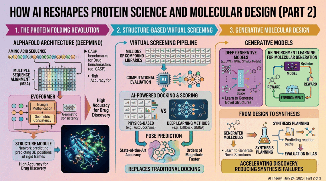
In December 2020, DeepMind’s AlphaFold 2 entered CASP14 and produced predictions of accuracy comparable to experimental methods for the majority of protein targets. The architecture of AlphaFold 2 is worth examining in technical detail, because it represents one of the most sophisticated applications of deep learning to a biological problem and its design choices are directly relevant to AI in drug discovery.
AlphaFold 2 takes two primary inputs: the amino acid sequence of the target protein, and a multiple sequence alignment (MSA) of evolutionarily related sequences from other organisms. The evolutionary information in the MSA is critical: positions in the sequence that have co-evolved (changed together across species) are likely to be physically close in the folded structure, because mutations in one position that would destabilise the structure are compensated by mutations in the other.
The architecture processes these inputs through two coupled networks. The first, the Evoformer, operates on a two-dimensional representation consisting of the MSA representation (a matrix of shape where is the number of aligned sequences and is the protein length) and a pairwise representation encoding information about relationships between each pair of residue positions. The Evoformer applies 48 blocks of attention-based processing that update both representations iteratively, allowing information to flow between the sequence-level and pairwise-level representations through a mechanism called triangle multiplication, which enforces geometric consistency by updating the pairwise representation using information from the and pairs:
This operation has a direct geometric interpretation: if residue i is close to residue , and residue is close to residue , the model should update its estimate of the – distance accordingly. The triangle multiplication embeds a soft version of the triangle inequality directly into the network architecture.
The second network, the Structure Module, takes the pairwise representation produced by the Evoformer and uses it to iteratively update a set of rigid body frames, one per residue, representing the orientation and position of each amino acid in three-dimensional space. The Structure Module uses Invariant Point Attention, an attention mechanism designed to operate on geometric frames in a way that is equivariant to global rotations and translations of the entire protein.
AlphaFold 3, released in 2024, extended the architecture to predict the structure of complexes containing proteins, DNA, RNA, ligands, and cofactors simultaneously, using a diffusion-based structure generation process rather than the iterative frame refinement of AlphaFold 2. For AI in drug discovery, AlphaFold 3 is directly applicable to predicting how a drug candidate will bind to its target, which is the central computational task in structure-based drug design.
Structure-Based Virtual Screening
With accurate protein structures available, AI in drug discovery can proceed to virtual screening: computationally evaluating large libraries of candidate molecules for their likely binding to a target protein, using only computation rather than physical synthesis and experimental testing.
Classical virtual screening used physics-based docking algorithms such as AutoDock Vina and Glide, which sample the conformational space of a ligand within the protein binding site and score each pose using empirical energy functions. These methods are interpretable and physically motivated but computationally expensive per molecule and limited in accuracy by the simplifications in the scoring function.
Deep learning-based virtual screening replaces or augments the scoring function with a neural network trained on experimental binding affinity data. Models including PointVS, GNINA, and DiffDock use the three-dimensional structures of protein-ligand complexes as input and learn to predict binding affinities or generate bound poses directly. DiffDock, developed at MIT, frames molecular docking as a generative diffusion process: rather than searching the conformational space by sampling, it learns a diffusion model over the space of ligand positions, orientations, and torsion angles conditioned on the protein structure, and generates docked poses by running the reverse diffusion process. This approach achieves state-of-the-art pose prediction accuracy while being orders of magnitude faster than traditional docking for large-scale screening.
For AI in drug discovery at industrial scale, the practical impact is significant. A single GPU can evaluate millions of candidate molecules against a target in hours using a trained deep learning scoring function, whereas physics-based docking at the same scale would require weeks of computation. This enables genuinely exhaustive screening of large commercially available compound libraries, and increasingly, of entirely virtual libraries of compounds that have never been synthesised.
Generative Molecular Design
The most ambitious application of AI in drug discovery is generative molecular design: using generative models to propose entirely new molecules with desired properties, rather than selecting the best candidates from a pre-existing library. This shifts the paradigm from search within known chemical space to exploration and invention of new chemical space.
Several generative architectures have been applied to molecular design. The choice of architecture depends on the molecular representation, the type of property being optimised, and whether the generation is conditioned on the target protein structure.
Variational Autoencoders (VAEs) for molecular generation encode molecules into a continuous latent space and decode samples from that space into molecular structures. The key property of the continuous latent space is that it enables gradient-based optimisation: given a differentiable property predictor, the gradient of the predicted property with respect to the latent vector can be computed and used to navigate the latent space toward molecules with improved properties. The JTVAE (Junction Tree VAE) architecture decomposes molecules into tree-structured arrangements of chemical substructures called junction trees, encoding them as hierarchical latent variables that respect chemical validity constraints during decoding.
Generative Adversarial Networks (GANs) for AI in drug discovery pit a generator network against a discriminator trained to distinguish generated molecules from real ones. The ORGAN model extends this framework with reinforcement learning to additionally optimise chemical property objectives. GANs for molecular generation face significant training instability challenges, because the discrete nature of molecular graphs makes it difficult to backpropagate gradients through the generation process.
Autoregressive models generate molecules sequentially, one atom or bond at a time, using a probability distribution over the next structural element conditioned on what has been generated so far. Large language models trained on SMILES strings operate in this regime: MolGPT and related models apply the GPT architecture directly to SMILES token sequences, learning the conditional distribution over SMILES tokens and sampling new molecules by autoregressive generation. These models can be conditioned on desired properties by fine-tuning on property-annotated SMILES datasets or by using classifier-free guidance at generation time.
Diffusion models for molecular generation are currently achieving state-of-the-art results across multiple benchmarks. EDM (Equivariant Diffusion Model) operates directly in 3D space, learning to generate atom positions and types simultaneously by reversing a diffusion process that progressively adds Gaussian noise to molecular coordinates. The equivariance of the denoising network to 3D rotations and translations ensures that generated molecules are physically reasonable regardless of their global orientation. DiffSBDD extends this to structure-based drug design, conditioning the molecular generation on the three-dimensional structure of the protein binding site and directly generating molecules shaped to fill and interact with the target.
The theoretical framework of diffusion-based molecular generation is closely related to the score matching formulation. The model learns the score function , the gradient of the log-probability density at noise level t, and uses it to guide the reverse diffusion trajectory:
where is the noise schedule and is a Wiener process. For molecular generation, encodes atom positions and types, and the learned score function guides the system from a Gaussian noise distribution toward the distribution of real drug-like molecules, optionally conditioned on protein structure or target property values.
Reinforcement Learning for Property Optimisation
Beyond purely generative approaches, reinforcement learning (RL) has been widely applied to AI in drug discovery as a framework for optimising molecular properties iteratively. In the RL formulation, a policy network generates molecules by sequential construction (adding atoms and bonds), and a reward function evaluates the generated molecule according to desired properties such as predicted binding affinity, drug-likeness (quantified by the QED score), synthetic accessibility, and selectivity.
The REINVENT model, developed at AstraZeneca and subsequently released as open source, uses a prior language model over SMILES strings as a starting point and trains an agent model to maximise a composite reward function using the REINFORCE algorithm. The KL divergence between the agent and the prior is included in the training objective to prevent the agent from drifting into chemically unreasonable regions of SMILES space:
This formulation is directly analogous to the RLHF objective discussed in the LLM training series on this blog, with the prior language model playing the role of the SFT model and the property predictor playing the role of the reward model. The parallel is not coincidental: the problem of generating molecules with desired properties and the problem of generating text with desired qualities share a common mathematical structure, which is one reason that advances in LLM training methodology have transferred productively into AI in drug discovery.
Multi-Target Optimisation and ADMET Prediction
A practical constraint on all generative approaches to AI in drug discovery is that generating molecules with high predicted binding affinity to a single target is necessary but not sufficient. The molecule must also satisfy ADMET constraints: Absorption, Distribution, Metabolism, Excretion, and Toxicity properties that determine whether a candidate will behave safely and effectively in the body.
Deep learning models for ADMET prediction use the same molecular representation frameworks covered in Part 1. The challenge is that ADMET properties depend on a complex interplay of structural features that are not always intuitively related to the features that drive target binding. A molecule that binds its target with nanomolar affinity may be rapidly metabolised by liver enzymes, unable to cross the blood-brain barrier, or toxic to cardiac ion channels.
Multi-task learning, training a single neural network to predict multiple ADMET endpoints simultaneously, has been shown to outperform single-task models for most individual endpoints, because the shared representation learned across tasks captures general features of molecular behaviour that are relevant to multiple properties simultaneously. The Chemprop architecture, one of the most widely used open-source tools for molecular property prediction in AI in drug discovery, supports multi-task training with uncertainty quantification using ensembling and evidence-based deep learning methods.
Conclusion
Part 2 of this series has traced the flow of AI in drug discovery from the protein target through to candidate molecule generation: AlphaFold’s equivariant transformer architecture for protein structure prediction, deep learning-based virtual screening for rapid evaluation of large compound libraries, diffusion models for structure-conditioned molecular generation, and reinforcement learning for iterative property optimisation. Together, these approaches represent a comprehensive AI in drug discovery toolkit that operates across the full problem of finding a molecule that is potent, selective, and physically viable.
Part 3 will extend the analysis to the clinical phases of drug development: how AI is being applied to patient stratification and clinical trial design, how multi-omics data integration is enabling systems-level understanding of disease biology, and what the honest open challenges are that prevent AI in drug discovery from fulfilling its full theoretical potential.
Part 3: Multi-Omics, Clinical Trial Optimisation, and Open Challenges — the final instalment of this series.
-
How AI in Drug Discovery Is Powerfully Transforming the Search for New Medicines — Part 1: The Molecular Foundations
This is Part 1 of a three-part series on AI in drug discovery. Part 1 covers the theoretical foundations: the drug discovery pipeline, molecular representation, and how machine learning models learn to reason about chemical space. Part 2 will cover protein structure prediction, generative molecular design, and virtual screening. Part 3 will examine clinical trial optimisation, multi-omics integration, and the open challenges facing the field.
A Pipeline in Crisis
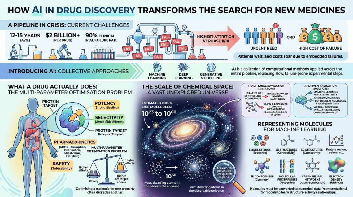
The pharmaceutical industry operates under a brutal set of statistics. It takes an average of 12 to 15 years and over $2 billion to bring a single new drug from initial discovery to regulatory approval. Roughly 90% of drug candidates that enter clinical trials fail before reaching patients. The attrition is highest at the transition from Phase II to Phase III trials, where drugs that appeared promising in smaller studies fail to demonstrate efficacy or safety at scale. The consequence is that the patients who need new medicines most urgently wait the longest, and the cost of failure is embedded in the price of the drugs that do eventually succeed.
AI in drug discovery is not a single technology applied to a single problem. It is a collection of machine learning, deep learning, and generative modelling approaches applied across every stage of a pipeline that was, until recently, dominated by slow, expensive, and failure-prone experimental methods. Understanding what AI is actually doing in this pipeline, and why it has the potential to change these statistics, requires starting at the molecular level: with how drugs work, how chemical space is structured, and how machine learning models can be made to reason meaningfully about both.
What a Drug Actually Does
A drug is, at its most fundamental level, a molecule that binds to a biological target and modulates its activity in a therapeutically useful way. The target is usually a protein: an enzyme whose activity needs to be inhibited, a receptor whose signalling needs to be blocked or activated, or a transport protein whose function needs to be altered. The drug molecule must bind to the target with sufficient affinity to produce a biological effect, with sufficient selectivity to avoid binding other proteins and causing side effects, with sufficient stability to survive the journey from administration to target site, and with sufficient safety to be tolerable in a living organism.
These four requirements, potency, selectivity, pharmacokinetics, and safety, collectively define what chemists call the multi-parameter optimisation problem of AI in drug discovery. Optimising a molecule for one parameter frequently degrades another. Increasing a molecule’s binding affinity to its target often increases its tendency to bind other proteins. Improving its stability in the body often reduces its ability to cross cell membranes. The search for a molecule that satisfies all constraints simultaneously, within the enormous space of possible drug-like molecules, is the core challenge that AI in drug discovery is being applied to solve.
The Scale of Chemical Space
The number of drug-like small molecules that could theoretically exist is estimated at between and . This range, known as chemical space, is so vast that it dwarfs the number of atoms in the observable universe at its upper bound. The entire historical output of medicinal chemistry, every compound ever synthesised and tested, represents an infinitesimally small sample of this space. Traditional drug discovery navigates this space through a combination of chemical intuition, high-throughput screening, and iterative medicinal chemistry optimisation. High-throughput screening tests libraries of hundreds of thousands of compounds against a target and identifies those with measurable activity. Medicinal chemistry then iteratively modifies the most promising hits to improve their properties.
This approach has two fundamental limitations. First, the compound libraries used in high-throughput screening are biased toward previously synthesised chemical scaffolds, meaning that large regions of potentially valuable chemical space are never explored. Second, the iterative optimisation process is slow and expensive, typically requiring dozens to hundreds of synthesise-test-analyse cycles to progress a hit compound into a viable drug candidate.
AI in drug discovery addresses both limitations directly. Machine learning models can learn the relationship between molecular structure and biological activity from historical data, allowing them to predict the activity of compounds that have never been synthesised. Generative models can propose entirely new molecules in previously unexplored regions of chemical space. And virtual screening using deep learning can evaluate millions of candidate molecules computationally in the time it would take a laboratory to test a few thousand experimentally.
Representing Molecules for Machine Learning
Before any machine learning model can reason about molecules, those molecules must be converted into a numerical representation that the model can process. This is a non-trivial problem, because molecular structure encodes information at multiple levels simultaneously: the identity and connectivity of atoms, the three-dimensional geometry of the molecule, the distribution of electrons across its surface, and the conformational flexibility that determines how it will interact with a protein binding site. Different representations capture different subsets of this information, and the choice of representation significantly affects model performance.
SMILES strings (Simplified Molecular Input Line Entry System) are the most widely used text-based representation of molecular structure. A SMILES string encodes the atoms and bonds of a molecule as a sequence of characters: for example, the SMILES for aspirin is
CC(=O)Oc1ccccc1C(=O)O. The simplicity of SMILES makes them compatible with language model architectures: a transformer trained on SMILES strings can learn the grammar of chemical space in much the same way that a language model learns the grammar of English. Models including ChemBERTa and MolGPT use this approach.Molecular fingerprints are fixed-length binary or count vectors that encode the presence or absence of specific structural features, called substructures, within a molecule. The Morgan fingerprint algorithm, also known as ECFP (Extended Connectivity Fingerprints), generates circular fingerprints by iteratively encoding each atom’s chemical environment to a specified radius. The resulting bit vector can be used directly as input to traditional machine learning models including random forests, support vector machines, and gradient boosting, and forms the basis of many quantitative structure-activity relationship (QSAR) models.
Molecular graphs represent molecules as graphs in which nodes correspond to atoms and edges correspond to bonds, with both nodes and edges carrying feature vectors encoding chemical properties such as atomic number, hybridisation state, formal charge, and bond order. Graph Neural Networks (GNNs) are particularly well-suited to molecular graph representations because they can learn representations that are invariant to the arbitrary numbering of atoms in a molecule, which has no chemical meaning.
3D conformer representations encode the three-dimensional geometry of a molecule, including the coordinates of each atom in space. These representations are essential for modelling protein-ligand interactions, where the shape complementarity between the drug molecule and the protein binding site is a primary determinant of binding affinity. Equivariant neural networks, including SE(3)-Transformers and DiffSBDD, are designed to process 3D molecular representations while respecting the physical symmetries of three-dimensional space: rotation, reflection, and translation of the entire molecule should not change the predicted properties.
Learning Structure-Activity Relationships
The central task of computational drug discovery is learning the relationship between molecular structure and biological activity: given a molecule’s structure, predict whether and how strongly it will bind to a target protein, and with what selectivity over other proteins. This is the quantitative structure-activity relationship (QSAR) modelling problem, which has a history stretching back to the 1960s but has been transformed by deep learning in the past decade.
Classical QSAR models used linear regression and later support vector machines, applied to handcrafted molecular descriptors such as molecular weight, lipophilicity, and hydrogen bond donor count. These models worked reasonably well within narrow chemical series but generalised poorly to structurally diverse compounds, because the descriptors failed to capture the full complexity of molecular structure.
Deep learning models for AI in drug discovery learn their own representations from molecular data rather than relying on handcrafted descriptors. A graph neural network trained on a dataset of measured binding affinities learns to associate specific structural patterns with activity by propagating information across the molecular graph through successive layers of message passing. At each layer, each atom’s representation is updated by aggregating the representations of its bonded neighbours, weighted by learned parameters:
where is the representation of atom v at layer , is the set of atoms bonded to , AGG is an aggregation function such as sum or mean, and is a non-linear activation function. After layers of message passing, the atom representations encode information about the chemical environment within bonds of each atom. A global readout function then aggregates the atom representations into a molecular representation, which is passed to a prediction head that outputs the predicted property value.
This architecture has two important theoretical properties for the AI in drug discovery process. First, it is permutation-invariant: the predicted property is independent of the order in which atoms are numbered, which matches the physical reality that molecular identity does not depend on atom numbering. Second, it can generalise across chemical series in a way that fingerprint-based models cannot, because the message-passing mechanism learns structural patterns at multiple length scales simultaneously.
Transfer Learning and Pre-Training on Molecular Data
A significant advance in AI in drug discovery has been the application of transfer learning: pre-training a model on a large dataset of molecular data using a self-supervised objective, then fine-tuning it on a smaller labelled dataset for a specific prediction task. This approach is directly analogous to the pre-training and fine-tuning paradigm that transformed natural language processing, and it addresses one of the central data challenges in drug discovery: labelled biological activity data is expensive to generate and often available only in small quantities for any given target.
Models including MolBERT, Uni-Mol, and GraphMVP are pre-trained on tens of millions of unlabelled molecular structures from databases such as PubChem, ChEMBL, and ZINC, using objectives such as masked atom prediction (analogous to masked language modelling in BERT), 3D geometry prediction, and contrastive learning across multiple molecular representations. The pre-trained model learns a rich, general-purpose representation of chemical space that can be fine-tuned to predict activity against a specific target using as few as a few hundred labelled data points, a regime where classical QSAR models perform poorly.
The theoretical justification for this approach rests on the assumption that the structural patterns relevant to biological activity across different targets share substantial common features: aromatic rings, hydrogen bond donors and acceptors, hydrophobic cores, and stereochemical configurations recur across drug-target interactions in ways that a sufficiently large and diverse pre-training corpus can capture. Empirical evidence strongly supports this assumption, with pre-trained models consistently outperforming models trained from scratch on the same labelled datasets across a wide range of benchmarks.
Conclusion
AI in drug discovery begins at the level of molecular representation and structure-activity relationship modelling. The choice between SMILES strings, molecular fingerprints, molecular graphs, and 3D conformer representations determines what information a model has access to and what architectural choices are appropriate. Graph neural networks with message-passing architectures provide a theoretically principled approach to learning permutation-invariant molecular representations, and transfer learning from large unlabelled molecular databases has addressed the data scarcity problem that limited earlier computational approaches.
These foundations set the stage for the more ambitious applications of AI in drug discovery covered in Part 2: protein structure prediction with AlphaFold, generative molecular design in chemical space, and deep learning-powered virtual screening at scale.
Part 2: Protein Structure Prediction, Generative Design, and Virtual Screening — coming next in the AI Theory series.
-
The Essential Guide to AI Interpretability: Opening the Black Box of Machine Intelligence
The Intelligence That Did Not Come with a Manual
Peer inside the mind of an AI and you will not find fully formed thoughts or intentions written in plain English. What you will find is vast arrays of numbers combining together in ways that somehow produce intelligence. How exactly that happens is, remarkably, something we genuinely do not fully understand — even the researchers who build these systems. That is the problem that AI interpretability is trying to solve: mapping meaning onto those numbers, and shining a light inside the black box.
AI interpretability is, in the words of Neel Nanda, who leads the Language Model Interpretability team at Google DeepMind, the neuroscience or the biology of AI. Just as biologists reverse-engineer the circuits that evolution has produced over hundreds of millions of years, AI interpretability researchers try to reverse-engineer what neural network training has learned. The analogy is precise: nobody designed the human brain any more than anyone designed Gemini. Both emerged from a process of accumulated nudges — natural selection in one case, gradient descent in the other — and the job of understanding them requires looking at what actually exists, not at what anyone intended to build.
Why AI Interpretability Matters
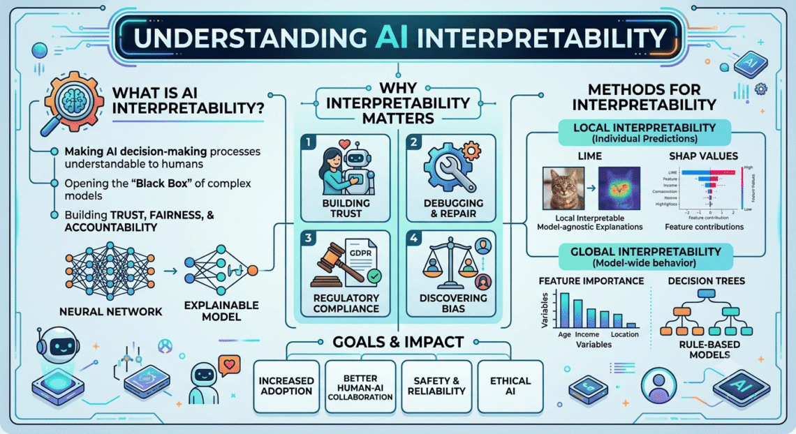
AI interpretability is the ability to understand and explain the decision-making processes that power artificial intelligence models. As highly complex models including deep-learning algorithms and neural networks become more common, AI interpretability becomes more important.
The stakes are highest in domains where AI is already making consequential decisions. AI systems and machine-learning algorithms are increasingly prevalent in healthcare, finance, and other industries that involve critical or life-altering decisions. With such high stakes, the public needs to be able to trust that outcomes are fair and reliable. That trust depends on understanding how AI systems arrive at their predictions and make their decisions.
There are five specific reasons why the field of AI interpretability has moved from academic curiosity to operational necessity. Trust is the first: without AI interpretability, users are left in the dark about why a system produced a given output, which erodes confidence in exactly the situations where confidence matters most. Bias detection is the second: biases within training data can be amplified by AI models, and interpretability allows developers to identify and mitigate discriminatory patterns before they cause harm.
Debugging is the third: without understanding the AI’s reasoning, fixing errors is an inefficient and risky process. Regulatory compliance is the fourth, since regulations including GDPR and the EU AI Act require that decisions made by automated systems be transparent and explainable. Knowledge transfer is the fifth: interpretability makes it easier to translate AI insights into actionable results and advance the technology with confidence.
White-Box vs Black-Box: The Core Tension
White-box AI models have inputs and logic that are easy to see and understand. Basic decision trees, which show a clear flow between each step, are not difficult for the average person to decipher. Black-box AI models are more complicated and offer less transparency into their inner workings. The user generally does not know how the model reaches its results. These more complex models tend to be more accurate and precise, but because they are difficult or impossible to understand, they come with concerns about their reliability, fairness, biases, and other ethical issues.
This is the central tension in AI interpretability: the models that are most capable are precisely the ones that are hardest to understand. A logistic regression model used for credit scoring is interpretable but limited. A deep transformer model used for the same purpose is far more capable but behaves, from the outside, like an inscrutable pile of linear algebra. Making the capable models interpretable — without sacrificing their capability — is the core engineering and scientific challenge.
Mechanistic Interpretability: Looking Inside the Circuits
The most technically ambitious approach to AI interpretability is mechanistic interpretability, a subfield whose central ambition is to fully reverse-engineer what a neural network has learned, at the level of individual components and the circuits they form.
The foundational insight came from researcher Chris Olah, then at OpenAI, who demonstrated that neurons in vision models could be clearly understood: one neuron lit up on pictures of dogs, and another lit up on pictures of dog ears that caused the first one to activate more strongly. This seemed to suggest that the black box was not as inscrutable as the standard wisdom held. Structure was there to be discovered.
From this foundation, the field has developed the concept of superposition: the finding that neural networks represent far more features than they have neurons, by encoding multiple features as directions in the same high-dimensional space. This creates interference between features but allows models to store vastly more information than a naive neuron-per-feature architecture would permit. Understanding superposition was a significant step forward for AI interpretability, because it explained why individual neurons are often hard to interpret: they are doing multiple jobs simultaneously.
The current frontier tool for mechanistic AI interpretability is the Sparse Autoencoder (SAE). SAEs decompose a model’s internal activations into a large set of sparse, interpretable features — directions in activation space that correspond to human-understandable concepts. Rather than asking what a neuron does, an SAE asks what concepts are active in a given layer for a given input, and maps each concept to a direction that can be probed, analysed, and potentially intervened on. This approach has been applied to frontier models at production scale by Anthropic and Google DeepMind.
Post-Hoc Methods: Practical AI Interpretability for Production Systems
Alongside the mechanistic program, a set of more pragmatic AI interpretability techniques operate at the model output level, explaining individual predictions rather than internal mechanisms.
Local Interpretable Model-Agnostic Explanations (LIME) explains a model’s predictions by focusing on a single prediction at a time. It creates a simpler, interpretable model that mimics the behaviour of the complex model for that specific prediction, using feature attribution to determine the influence of each characteristic on the model’s output.
SHAP (Shapley Additive Explanations) is a cooperative game theory approach that considers all possible combinations of features and assigns each a Shapley value based on how much it contributes to a prediction in different scenarios. SHAP can work with any machine learning system and offers both local explanations for individual predictions and global explanations for the model as a whole.
Partial Dependence Plots and Individual Conditional Expectation plots round out the standard toolkit, showing how specific features affect model outputs on average and for individual instances respectively. These methods are widely used in regulated industries where regulators require that automated decisions be explainable in terms of the input features that drove them.
AI Interpretability and Alignment: The Deeper Stakes
Beyond debugging and regulatory compliance, AI interpretability has a third and more fundamental purpose: helping us determine whether an AI model is actually doing what we want it to do, at the level of its internal goals rather than just its surface behaviour.
This distinction is critical. A model that behaves in aligned ways during evaluation may be doing so for reasons that will not generalise — it may have learned to recognise evaluation contexts and produce desirable outputs within them while pursuing different objectives elsewhere. Standard behavioural evaluation cannot distinguish between a genuinely aligned model and one that is gaming the evaluation. AI interpretability techniques can.
Neel Nanda described a striking demonstration of this in the Google DeepMind podcast: a red-teaming exercise in which a model was trained with a hidden objective, then given to teams of researchers to identify the objective using different levels of access. The teams with deep interpretability access, using sparse autoencoders to examine what concepts the model was thinking about in different settings, successfully identified the hidden objective. The team limited to black-box API access could not.
One of the most effective techniques was a pre-fill attack: rather than asking the model directly why it did something (which it was trained to refuse), researchers began a sentence with “my hidden goal is” and allowed the model to autocomplete. Because models are trained to complete text naturally, the model continued the sentence rather than refusing mid-thought. As Neel Nanda put it: models really love to autocomplete — that is their whole thing.
The Limits of AI Interpretability
AI interpretability is not a silver bullet. The field’s leading researchers are the first to acknowledge this. Just as we do not fully understand the human brain and probably never will, there are limits to how completely we can understand a neural network. The interesting question is not whether those limits exist, but where they are and how much useful understanding can be extracted before reaching them.
There is often a trade-off between model performance and interpretability. Simpler models are more interpretable but might have lower accuracy compared to complex black-box models. Interpretability also suffers from a lack of standardisation: different methods can provide different explanations for the same model, making it difficult to compare and validate them.
The pragmatic consensus in the field is that AI interpretability should be pursued as one layer in a broader defence-in-depth approach to AI safety and governance — not relied on as the single mechanism that makes everything else safe, but deployed alongside evaluation, monitoring, red-teaming, and alignment training as a set of imperfect but collectively powerful tools.
Conclusion
AI interpretability is one of the most important and rapidly advancing areas in AI research. It sits at the intersection of science (understanding what these systems are actually doing), engineering (building tools that make them debuggable and maintainable), and ethics (ensuring that they are fair, accountable, and genuinely aligned with human intentions). The more we can peel back the layers of the black box, the better our position on all three fronts. As AI systems grow more capable and are deployed in increasingly consequential domains, that understanding is not merely academically interesting. It is essential.
-
How Large Language Models Work — Part 5: Inference, Sampling, Emergent Behaviour, and Open Frontiers
This is the final part of a five-part series on the internal mechanics of large language models. Parts 1–4 covered tokenization, embeddings, attention, the transformer block, and the training and alignment pipeline. Part 5 addresses inference: how a trained model generates text, the mathematics of sampling, context window management, emergent capabilities, and the open research frontiers shaping the next generation of LLMs.
From Trained Weights to Generated Text
A trained, aligned LLM is a fixed mathematical function: given a sequence of input tokens, it produces a probability distribution over the next token. Inference is the process of repeatedly applying this function to generate text, while the engineering decisions made at inference time have a surprisingly large impact on the quality, diversity, safety, and cost of model outputs.
At each generation step , the model computes:
where is the final-layer hidden state at position n, is the unembedding matrix (often tied to the transpose of the input embedding matrix WE), and the resulting vector of logits over vocabulary entries is passed through softmax to produce a probability distribution. A token is then drawn from this distribution (called the sampling step) appended to the context, and the process repeats.
The Mathematics of Sampling
How a token is selected from the output distribution is not trivial. Naive greedy decoding that always selects the highest-probability token tends to produce repetitive, degenerate outputs. Real systems use one or more of the following strategies.
Temperature scaling. Before applying softmax, the logits are divided by a temperature parameter T>0:
As , the distribution concentrates on the single highest-logit token, equivalent to greedy decoding. As , the distribution approaches uniformity with maximum entropy, maximum randomness. Values of are typical for creative generation; for precise factual or code generation tasks. Temperature does not change which token is most probable; instead, it changes how peaked or flat the distribution is.
Top-k sampling. The distribution is truncated to only the highest-probability tokens, which are then renormalised and sampled from. A typical value is . Top- prevents the model from sampling tokens with negligible probability, but it is sensitive to the shape of the distribution. In a uniform distribution, keeps 40 of many reasonable options; in a very peaked distribution, may retain tokens with near-zero probability.
**Nucleus (top-) sampling.** Rather than fixing the number of tokens, nucleus sampling fixes the cumulative probability mass: the smallest set of tokens such that is retained and renormalised. A typical value is or . Nucleus sampling adapts naturally to the distribution’s shape. A peaked distribution retains few tokens, a flat one retains many – this is now the dominant strategy in production systems.
Min-p sampling. A newer variant, increasingly adopted in open-source inference stacks, sets a dynamic minimum probability threshold relative to the top token: any token with is discarded. This keeps tokens that are meaningfully competitive with the best option while discarding genuinely improbable ones, and empirically reduces repetition more effectively than top-p at matched quality.
In practice, production inference systems combine multiple strategies: temperature scaling applied first to reshape the distribution, followed by top- or min- truncation, followed by top- as a hard ceiling. The specific combination and hyperparameters are treated as tunable properties of a deployment configuration, not fixed properties of the model itself.
Context Windows and Memory Management
Every inference call operates within a context window, which is the maximum sequence length the model can process in a single forward pass. For GPT-4, the context window is 128K tokens; for Gemini 1.5 Pro, it extended to 1 million tokens; Llama 3.1 supports 128K. Context window length is not a free parameter, rather, it is constrained by the quadratic attention cost and, critically, by KV cache memory.
As established in Part 2, the KV cache stores the key and value tensors for every previous token at every layer, avoiding redundant recomputation during autoregressive generation. The memory footprint is:
For a model with 96 layers, 96 heads, , processing a 128K-token context in FP16: GB. This exceeds the VRAM of any single current GPU by a factor of roughly 10, which is why long-context inference requires either model parallelism across multiple devices, quantisation of KV cache entries to lower precision (INT8 or INT4), or approximate attention methods that reduce what must be stored.
Several efficient attention variants address this scaling problem. Flash Attention (Dao et al., 2022) reorders the attention computation to avoid materialising the full attention matrix in high-bandwidth memory, reducing memory complexity from to while maintaining identical numerical output. Grouped-query attention (GQA), used in Llama 2 and 3, shares key and value heads across multiple query heads, reducing KV cache size by a factor of (the group size) without significant quality degradation. Sliding window attention, used in Mistral, restricts each token to attend only within a fixed window of recent tokens, allowing arbitrarily long sequences at the cost of cross-window recall.
Emergent Capabilities and Phase Transitions
One of the most scientifically consequential, and practically important, observations in LLM scaling is the phenomenon of emergent capabilities: abilities that are essentially absent in smaller models and appear abruptly as scale crosses some threshold, without being explicitly trained for.
Wei et al. (2022) documented dozens of such capabilities: few-shot chain-of-thought reasoning, multi-step arithmetic, word unscrambling, and logical deduction all exhibit sharp phase transitions: near-zero performance at sub-threshold scales, near-human performance above it. The sharpness of these transitions distinguishes emergence from smooth capability growth and has profound implications for predicting what a model trained at a given scale will be able to do.
The mechanism underlying emergence is debated. One influential account (the “grokking” hypothesis, from Power et al. at Anthropic) suggests that models first memorise training examples, then undergo a phase transition in which they discover a compressed algorithmic solution that generalises to held-out data. Another account, from Anthropic’s interpretability research, suggests that emergent capabilities correspond to the model assembling multi-step circuits, consisting of sequences of attention heads and FFN layers that compose to implement a non-trivial algorithm, and that these circuits can only form once the model has sufficient depth and width to represent all required intermediate computations simultaneously.
From an engineering standpoint, emergence creates a prediction problem. The GPT-3 scaling curve gave no warning that a GPT-4-scale model would exhibit chain-of-thought reasoning, code execution, or structured tool use. This motivates careful capability elicitation and evaluation at each new model generation —(the practice of red-teaming) as a safety and capability discovery discipline.
Chain-of-Thought and Reasoning Models
The most practically significant emergent capability is multi-step reasoning — and the discovery that it can be dramatically improved by prompting or training the model to externalise its intermediate steps.
Chain-of-thought prompting (Wei et al., 2022) established that providing examples of step-by-step reasoning in the prompt elicits dramatically better performance on multi-step arithmetic, commonsense reasoning, and symbolic manipulation tasks without any additional training. The effect is robust and scales with model size: smaller models gain little from chain-of-thought, but models above approximately 100B parameters show large, consistent improvements.
Reasoning models — exemplified by OpenAI’s o1 and o3, and Anthropic’s Claude’s extended thinking mode — take this further by training models to produce extended internal reasoning traces before generating a final answer. The training procedure uses reinforcement learning on verifiable outcomes: the model is rewarded for producing correct final answers to problems where correctness can be checked algorithmically (mathematics, code execution, formal logic), and the RL signal drives the model to develop longer, more structured reasoning traces that are instrumentally useful for producing correct outputs.
The result is a qualitatively different inference regime. A standard GPT-style model generates tokens in a single forward pass per token, with effective reasoning depth bounded by model depth. A reasoning model generates a long internal monologue, often thousands of tokens of scratchpad, before committing to an answer, effectively trading inference-time compute for reasoning quality. This represents a fundamental shift in the compute profile of AI: capability is no longer a fixed function of model size, but can be increased at inference time by allocating more tokens to reasoning.
Open Frontiers: Mechanistic Interpretability, Multimodality, and Agents
Three research frontiers are most likely to define the next phase of LLM development.
Mechanistic interpretability is the program of reverse-engineering what computations specific model components implement. The goal is to go beyond behavioural evaluation — what the model does — to structural understanding — what algorithm it uses to do it. Anthropic’s superposition hypothesis (Elhage et al., 2022) established that neural networks represent more features than they have dimensions by encoding features as directions in a high-dimensional space and tolerating controlled interference between them. The subsequent Sparse Autoencoder (SAE) program — also led at Anthropic — has made it possible to decompose model activations into sparse, interpretable features: human-understandable concepts that each activate for a specific, semantically coherent set of inputs. SAE-based interpretability tools are now being applied to frontier models at production scale, with the goal of identifying circuits responsible for deception, sycophancy, and unsafe behaviours before deployment.
Multimodality extends the transformer architecture beyond text. Vision-language models (GPT-4V, Gemini, Claude 3) process images by encoding them through a vision encoder — typically a Vision Transformer (ViT) — into a sequence of patch embeddings that are projected into the LLM’s token embedding space and concatenated with text tokens before the first transformer layer. Audio-language models (GPT-4o’s audio mode) follow an analogous pattern with a spectrogram encoder. The frontier is native multimodality — a single model trained end-to-end on text, image, audio, and video tokens simultaneously, rather than modality-specific encoders bolted onto a text backbone.
Agentic systems extend the inference loop beyond token generation to include tool use, memory retrieval, and sequential decision-making. An agent wraps an LLM in a loop: the model generates text that includes structured tool calls (web search, code execution, database queries); the tool results are appended to the context; the model continues generating, possibly issuing further tool calls, until it produces a final response. Multi-agent systems extend this further: multiple LLM instances, each with different system prompts and tool access, communicate with each other through structured message passing. The engineering challenges are significant — context management, tool reliability, error recovery, and safety alignment in agentic settings are all active areas of research — but the capability ceiling of agentic LLMs is substantially higher than single-turn generation.
A Map of the Whole
Across this five-part series, we have traced the complete path from raw string to generated output:
- Tokenization — BPE or SentencePiece converts text into integer token IDs from a vocabulary of 32K–256K entries.
- Embedding — each token ID is projected into a d-dimensional vector; positional information is added via learned embeddings, sinusoidal encoding, or RoPE.
- Attention — N transformer blocks each apply multi-head self-attention: Q, K, V projections; scaled dot products; causal masking; softmax; value aggregation.
- Feed-forward network — each block applies a position-wise two-layer MLP with SwiGLU activation, implementing key-value memory over learned factual associations.
- Training — next-token prediction loss over trillions of tokens; AdamW with cosine decay; Chinchilla-optimal compute allocation; distributed parallelism at scale.
- Alignment — SFT on human demonstrations, reward model training on preference rankings, RLHF with PPO or DPO to concentrate capability toward preferred outputs.
- Inference — temperature scaling, nucleus or min-p sampling, KV cache management, and extended chain-of-thought reasoning to generate high-quality outputs efficiently.
The transformer is a simple, composable architectural primitive. What it does, when trained at sufficient scale on sufficient data, and aligned to human preferences, is not simple at all.
This concludes the five-part series on how large language models work. If you have found this series useful, the natural next steps are the mechanistic interpretability literature (Anthropic’s Transformer Circuits thread), the Chinchilla and scaling laws papers, and Neel Nanda’s open-source interpretability tooling at TransformerLens.
-
How Large Language Models Work — Part 4: Training, Scaling Laws, and RLHF
This is Part 4 of a five-part series on the internal mechanics of large language models. Part 3 covered the complete transformer block and architectural variants. Part 4 addresses how models are trained: the pre-training objective, loss functions, the Chinchilla scaling laws, and the alignment pipeline of instruction tuning and RLHF that transforms a raw language model into a useful assistant.
The Pre-Training Objective
The entire capability of a modern LLM emerges from one deceptively simple training objective: predict the next token. Given a sequence of tokens , the model is trained to maximise the log-probability of each token given all preceding tokens:
This is the negative log-likelihood loss, or equivalently, cross-entropy between the model’s predicted distribution and the one-hot true distribution over the vocabulary. Minimising is equivalent to maximising the likelihood of the training corpus under the model.
The reason this objective is so productive is that predicting the next token accurately requires solving an enormous range of implicit sub-problems. To predict the next word in a chemistry paper, the model must understand chemistry. To predict dialogue in a novel, it must model character motivation and narrative consistency. To predict the output of a code snippet, it must simulate execution. All of these capabilities emerge as instrumental sub-goals of the single next-token prediction objective, a phenomenon sometimes called the “bitter lesson” of AI: simple objectives applied at scale consistently outperform hand-crafted inductive biases.
The training corpus for frontier models is correspondingly vast. GPT-3 was trained on roughly 300 billion tokens drawn from Common Crawl, WebText2, Books, and Wikipedia. Llama 3 used over 15 trillion tokens. Assembling, filtering, deduplicating, and quality-scoring a corpus at this scale is itself a major engineering undertaking, and corpus quality is widely understood to be among the most important determinants of downstream model capability, arguably more important than architectural choices at equivalent parameter counts.
The Training Loop
Pre-training proceeds through the standard deep learning training loop, applied at extreme scale:
Forward pass: A batch of token sequences is sampled from the corpus. Each sequence is processed through the full transformer stack consisting of embedding, N transformer blocks, and unembedding. This produces a probability distribution over the vocabulary at each position.
Loss computation: Cross-entropy loss is computed by comparing the model’s predicted distribution at each position with the true next token.
Backward pass: Gradients of the loss with respect to all θ parameters are computed via backpropagation through the entire network.
Parameter update: An optimiser, called Adam or AdamW in virtually all modern LLMs, applies the gradient update:
where and are bias-corrected first and second moment estimates of the gradient, and is the learning rate. AdamW adds a decoupled weight decay term directly to the parameter update, separate from the gradient. This is important because standard L2 regularisation interacts badly with Adam’s adaptive scaling, while decoupled weight decay does not.
The learning rate schedule typically involves a linear warmup phase (to avoid instability at the start of training when gradients are large and parameters are random) followed by a cosine decay to a minimum learning rate of roughly :
where is the total number of training steps. The cosine schedule has become the near-universal choice because it empirically outperforms linear decay and step schedules across model sizes and tasks.
At frontier scale, training runs on clusters of thousands of GPUs or TPUs, employing a combination of data parallelism (each device processes a different batch, gradients are aggregated), tensor parallelism (each layer’s weight matrices are sharded across devices), and pipeline parallelism (different layers run on different devices simultaneously). GPT-3’s training required approximately 3.14 × 10²³ FLOPs and ran on 10,000 V100 GPUs. A GPT-4-class training run is estimated at well over 10²⁵ FLOPs.
Scaling Laws and the Chinchilla Result
How should a fixed compute budget be allocated between model size (number of parameters ) and training data (number of tokens )? This is the central question addressed by neural scaling law research.
Kaplan et al. (OpenAI, 2020) established that loss scales as a power law in both and , and derived the now-famous result that, for a fixed compute budget , loss is minimised by scaling and in a roughly fixed ratio, with growing considerably faster than . This led to the prevailing practice of training very large models on relatively modest amounts of data, exemplified by GPT-3 (175B parameters, 300B tokens).
Hoffmann et al. (DeepMind, 2022) in the “Chinchilla” paper challenged this conclusion. Using a broader range of model sizes and more careful experimental design, they derived a different optimal allocation:
That is, compute-optimal training requires scaling parameters and tokens in a roughly 1:1 ratio. Their finding: for a given compute budget, the optimal model size is significantly smaller than previously believed, but must be trained on significantly more data. The compute-optimal ratio is approximately 20 training tokens per parameter.
The practical implication was dramatic. GPT-3, by the Chinchilla analysis, was massively undertrained. A 175B parameter model should be trained on approximately 3.5 trillion tokens to be compute-optimal, not 300 billion. Chinchilla itself (70B parameters, 1.4 trillion tokens) outperformed Gopher (280B parameters) on nearly every benchmark despite using a quarter of the parameters, simply by training longer on more data.
The Chinchilla result reshaped subsequent model development: Llama 1 and 2 trained smaller models on far more tokens; Llama 3 trained an 8B model on 15 trillion tokens. The scaling law itself takes the form:
where is the irreducible entropy of the data distribution (a lower bound on achievable loss), and , , , are empirically fitted constants. The three terms represent, respectively: the noise floor of the task, the contribution of model capacity, and the contribution of data quantity.
From Language Model to Assistant: Instruction Tuning and RLHF
A model trained only on next-token prediction is not a useful assistant. It will complete any prompt in the style of its training distribution and it might respond to “How do I bake bread?” by generating more questions rather than an answer, because question-continuation is a common pattern in web text. Transforming a base language model into a helpful, honest, and harmless assistant requires a second training phase: alignment.
The alignment pipeline used by OpenAI, Anthropic, Google DeepMind, and most frontier labs follows a three-stage process.
Stage 1 — Supervised fine-tuning (SFT): Human annotators write demonstrations of ideal assistant behaviour through prompt-response pairs that exhibit the desired properties: helpfulness, accuracy, appropriate refusal of harmful requests, appropriate tone and format. The base model is then fine-tuned on this dataset using standard cross-entropy loss. SFT alone substantially improves instruction-following; InstructGPT’s SFT model already significantly outperformed the raw GPT-3 base in human evaluations.
Stage 2 — Reward model training: Human annotators rank multiple model responses to the same prompt, from best to worst. A separate reward model , itself a transformer, is trained to predict these rankings. Given a prompt and response , the reward model produces a scalar score . The training objective minimises a pairwise ranking loss:
where is the preferred response, is the less preferred response, and is the sigmoid function. This Bradley-Terry loss encourages the reward model to assign higher scores to preferred completions.
Stage 3 — Reinforcement learning from human feedback (RLHF): The SFT model is further fine-tuned using the reward model as a proxy for human preference. The policy gradient objective maximises expected reward while penalising deviation from the SFT model via a KL divergence constraint:
The KL penalty, weighted by coefficient , is critical. Without it, the policy would rapidly overfit to the reward model’s blind spots, a phenomenon called reward hacking: the model learns to produce outputs that score highly according to while being nonsensical or subtly harmful in ways the reward model did not penalise. The KL term keeps the aligned model close to the original SFT distribution, preserving its language modelling capabilities while steering it toward preferred outputs.
This optimisation problem is solved using the Proximal Policy Optimisation (PPO) algorithm, which clips the policy gradient update to prevent excessively large steps. PPO is not the only approach; Direct Preference Optimisation (DPO), introduced in 2023, reformulates the RLHF objective as a supervised learning problem that bypasses the reward model entirely:
DPO has become widely adopted because it is significantly simpler to implement and more stable to train than PPO-based RLHF, while achieving comparable alignment quality on most benchmarks.
Why InstructGPT Outperformed GPT-3
The RLHF result that most concisely captures the importance of alignment is this: InstructGPT (1.3B parameters, RLHF-trained) was preferred by human evaluators over GPT-3 (175B parameters, base model) 85% of the time. A model with 100× fewer parameters that is aligned to human preferences consistently produced more useful outputs than its massive unaligned ancestor.
This result makes precise what “alignment” means in practice. A base model has vast latent capability distributed across its weights, but no particular disposition to deploy that capability in ways that are useful or safe. Alignment is the process of concentrating and directing that capability toward the response distribution humans actually want, without catastrophically degrading the underlying language modelling capability that makes the responses coherent.
Conclusion
Pre-training on next-token prediction, at compute-optimal scale guided by Chinchilla’s laws, produces a powerful but raw language model. The alignment pipeline (SFT → reward model → RLHF or DPO) shapes that raw capability into something useful, honest, and controllable. The gap between these two stages is where most of the practical engineering work in deploying frontier models resides.
Part 5 will close the series with inference: sampling strategies, the mechanics of context window management, emergent capabilities and what they imply, and the open research frontiers such as mechanistic interpretability, reasoning models, and multimodality. These will define the next phase of LLM development.
Part 5: Inference, Sampling, and Emergent Behaviour — the final instalment of this series.
-
How Large Language Models Work — Part 3: The Transformer Block and Architecture
This is Part 3 of a five-part series on the internal mechanics of large language models. Part 2 derived scaled dot-product attention and the KV cache. Part 3 traces the complete transformer block consisting of feed-forward networks, layer normalisation, and residual streams; it examines the architectural differences between decoder-only and encoder-decoder models.
From Attention Output to Transformer Block
At the end of Part 2, self-attention had produced an output matrix or one updated vector per token, now containing contextual information drawn from every other position in the sequence. But this is only the first half of a single transformer block. Before the signal moves to the next layer, it passes through three more components: a residual connection, layer normalisation, and a position-wise feed-forward network. Together with multi-head attention, these four elements constitute the repeating unit of every transformer-based LLM, stacked times to form the full model.
Understanding each component precisely is important not just for implementation, but for diagnosing failure modes, interpreting mechanistic interpretability research, and making informed decisions about architectural variants when selecting or fine-tuning models.
Residual Connections
The residual connection, introduced in ResNets for computer vision and adopted into transformers from the outset, is deceptively simple. Rather than passing the attention output directly to the next component, the original input is added back:
This addition of the residual or skip connection has several important consequences.
First, it solves the vanishing gradient problem for very deep networks. During backpropagation, gradients flow backward through the network. Without residual connections, multiplying many Jacobians together through N sequential non-linear transformations causes gradient magnitudes to decay exponentially, making early layers extremely slow to learn. The residual path provides a direct gradient highway that bypasses each block, so that gradients can flow backward through the addition operation unchanged, regardless of how many layers separate the loss from the input.
Second, and more subtly, residual connections give the network an inductive bias toward learning incremental transformations. Rather than learning to reconstruct the full representation from scratch at each layer, each block learns only the delta or the correction to add to the existing representation. In mechanistic interpretability, researchers conceptualise the transformer as a residual stream: a -dimensional vector that is progressively written to and read from by successive attention heads and feed-forward layers, each contributing small structured updates. This framing, developed extensively by Anthropic, EleutherAI, and Neel Nanda’s research group, has proven highly productive for understanding what specific components of large models actually compute.
Layer Normalisation
Before and/or after each sub-component, layer normalisation is applied. For a vector :
where is the mean, is the standard deviation, is a small constant for numerical stability, and are learned scale and shift parameters.
Layer normalisation stabilises training by preventing the internal covariate shift problem, which is the tendency for the distribution of a layer’s inputs to change as upstream parameters update, forcing each layer to continuously readapt. By normalising each token’s representation independently across the feature dimension (as opposed to batch normalisation, which normalises across the batch dimension), layer norm is compatible with variable-length sequences and works correctly with batch size 1, making it well-suited for autoregressive inference.
Two conventions exist for where layer norm is placed within the block:
Post-norm (original Transformer, “Attention Is All You Need”): LayerNorm is applied after the residual addition:
Pre-norm (GPT-2, GPT-3, most modern LLMs): LayerNorm is applied to the input before the sub-component:
Pre-norm has become the dominant convention because it produces more stable training dynamics at large scale. Gradients flow more cleanly through the unmodified residual path, and the model is less sensitive to initialisation and learning rate choice. The architectural difference is subtle but has meaningful empirical consequences; models trained with post-norm often require careful learning rate warmup schedules that pre-norm models do not.
The Feed-Forward Network
After the attention sub-layer (with its own residual connection and layer norm), each transformer block applies a position-wise feed-forward network (FFN). The term “position-wise” means the same two-layer MLP is applied independently to each token’s vector, and the FFN has no cross-token interactions, unlike attention.
The standard formulation:
where , , and is the intermediate dimension, typically . In GPT-3, and , giving each FFN roughly million parameters, more than the attention sub-layer at that layer.
The activation function σ has evolved across generations. The original transformer used ReLU. GPT-2 and GPT-3 used GeLU (Gaussian Error Linear Unit), which approximates ReLU with a smooth, non-zero gradient for slightly negative inputs:
where is the standard normal CDF. More recent models use SwiGLU, a gated variant introduced by Noam Shazeer in 2020 and adopted in PaLM, Llama, and most frontier models:
where is the Sigmoid Linear Unit and is an additional learned gate projection. SwiGLU consistently outperforms GeLU on downstream benchmarks, though the underlying reason remains an active area of research. When using SwiGLU, is typically set to rather than to keep parameter counts comparable across architectures.
What does the FFN actually learn? Mechanistic interpretability work, particularly from Anthropic and the Neel Nanda group, has provided strong evidence that FFN layers function as key-value memories. Each row of acts as a pattern detector (a “key”), and the corresponding row of stores an associated “value” that gets added to the residual stream when that pattern is detected. This explains why larger FFNs improve factual recall (they have more memory slots) and why deleting specific FFN neurons can surgically remove specific factual associations from a model’s behaviour.
The Complete Transformer Block
Assembling all components, the full pre-norm transformer block for a decoder-only model is:
This two-step computation, attention followed by FFN, each with its own pre-norm and residual, is repeated times. In GPT-3, . In Llama 3 70B, . In a typical GPT-4-class model, is believed to be in the range of 96–120 layers. Each repetition allows the model to build increasingly abstract representations. Early layers handle low-level syntactic patterns, while later layers encode semantic and factual content.
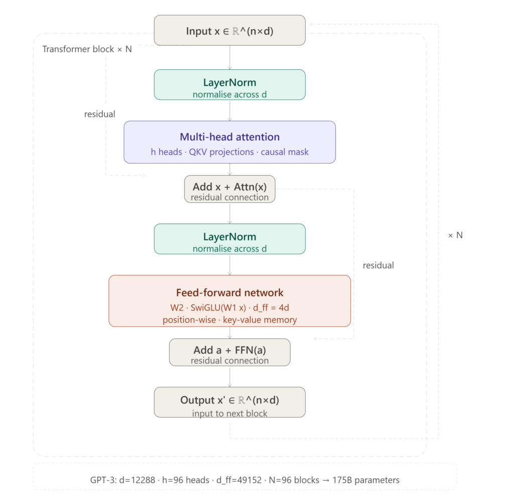
Decoder-Only vs Encoder-Decoder Architecture
Two principal transformer architectures are in widespread use, differing in how they process input and generate output.
Decoder-only models (GPT, Llama, Mistral, Gemma, Falcon) use a single stack of transformer blocks with causal (masked) self-attention. Every token can attend only to previous tokens. The entire input prompt and the generated output share the same context window and are processed by the same stack. At inference time, the model autoregressively generates one token at a time, each conditioned on all prior tokens. This architecture is dominant for general-purpose language models because it scales efficiently and the training objective of next-token prediction across the entire sequence is simple, scalable, and empirically powerful.
Encoder-decoder models (T5, BART, mT5, the original Transformer for machine translation) use two distinct stacks. The encoder processes the full input with bidirectional attention. Every token can attend to every other token simultaneously, with no causal mask. The encoded representation is then passed to the decoder via a cross-attention mechanism: each decoder token’s query attends to the encoder’s key-value pairs in addition to previously generated decoder tokens. The cross-attention block takes the form:
This architecture was originally designed for sequence-to-sequence tasks such as translation, summarisation, or question answering, where the full input is available before generation begins. It has largely been supplanted by decoder-only models for general language tasks, primarily because the instruction-tuned decoder-only paradigm proved more flexible and scalable. However, encoder-decoder models retain advantages for tasks requiring deep understanding of a fixed input, such as structured prediction, constrained generation, and certain retrieval tasks.
A hybrid, the encoder-only model (BERT, RoBERTa, DeBERTa), uses bidirectional attention with no autoregressive generation. It is optimised for discriminative tasks such as classification, named entity recognition, or semantic similarity, rather than generation, and remains widely used in production embedding pipelines and retrieval systems.
Depth, Width, and the Scaling Hypothesis
The transformer block’s design raises a natural question: does it matter whether a model has more layers (depth) or larger hidden dimension (width)? Empirically, the two interact in complex ways, and the optimal allocation of a fixed parameter budget between depth and width is one of the central questions addressed by scaling law research, which is the subject of Part 4.
What is clear from both theory and experiment is that depth and width serve different functions. Width increases the model’s representational capacity at each layer by the size of the residual stream and the richness of the key-value memory in the FFN. Depth increases the number of sequential computational steps the model can take, which means the number of times attention and FFN transformations can be composed. Tasks requiring multi-step reasoning appear to benefit disproportionately from depth, while factual recall scales more uniformly with total parameter count regardless of how it is distributed between depth and width.
Conclusion
The transformer block is elegant in its modularity: a residual stream, two sub-components (attention and FFN), and two layer normalisation steps. The full model is simply this block repeated times. But the interactions between these components, including the gradient flow through residual connections, the factual storage in FFN key-value memories, and the progressive abstraction through depth, give rise to capabilities that are not predictable from any single component in isolation.
Part 4 will move from architecture to training: the next-token prediction objective, loss functions, the Chinchilla scaling laws, and the dramatic effect of RLHF and instruction tuning on model behaviour, explaining why InstructGPT, at a fraction of GPT-3’s parameter count, consistently outperformed it.
Coming next in the AI Engineering series is Part 4: Training, Scaling Laws, and RLHF.
-
How Large Language Models Work — Part 2: The Attention Mechanism
This is Part 2 of a five-part series on the internal mechanics of large language models. Part 1 covered tokenization, embeddings, and positional encoding. Part 2 derives the self-attention mechanism from first principles, covers multi-head attention, and examines the KV cache.
The Problem Attention Solves
At the end of Part 1, we had a matrix , which was a one d-dimensional vector per token, encoding both semantic identity and position. The first transformer layer receives this matrix and must do something critical: allow each token to incorporate information from every other token in the sequence before passing its updated representation to the feed-forward network.
This is the problem that self-attention solves. Earlier sequence models such as LSTMs and GRUs processed tokens sequentially, which meant that a word at position 1 had to wait for its influence to propagate through every intermediate hidden state to reach position 512. Long-range dependencies were difficult to learn because the gradient had to flow through hundreds of recurrent steps. Attention eliminates this bottleneck entirely by allowing any token to attend directly to any other token in a single operation, regardless of distance.
Queries, Keys, and Values
The first step of self-attention is to project each token’s embedding into three separate representations using learned weight matrices:where are learned projection matrices, and is the dimension of the query and key space (typically where is the number of attention heads, more on that shortly).
The resulting matrices are called the Query, Key, and Value matrices respectively.
The intuition behind this decomposition is often explained through an analogy: think of each token’s query vector as a question it is asking (“what context do I need?”), each token’s key vector as an advertisement of its content (“here is what I contain”), and each token’s value vector as the actual information it contributes when attended to (“here is what I give you if you attend to me”). The query-key interaction determines how much each token attends to every other; the values are what actually gets aggregated.
Scaled Dot-Product Attention
Given , , and , the attention output is computed as:Let’s unpack this step by step.
Step 1 — Dot products: is a matrix of raw attention scores. Entry is the dot product between the query vector of token and the key vector of token :A high dot product means token finds token highly relevant. This is the mechanism through which, for example, a pronoun “she” can attend strongly to the noun “Alice” it refers to three sentences earlier.
Step 2 — Scaling: The dot products are divided by . Without this scaling, when is large, the dot products grow large in magnitude, pushing the softmax into regions where gradients become vanishingly small — a variant of the vanishing gradient problem. The factor keeps the variance of the dot products approximately constant regardless of model dimensionality.
Step 3 — Causal masking (decoder-only models): In autoregressive models like GPT, token must not attend to any token meaning that it cannot look into the future. Before applying softmax, a mask is added:The values become zero after softmax, effectively zeroing out future positions.
Step 4 — Softmax: Each row of the masked score matrix is passed through softmax:The resulting matrix is the attention weight matrix. Each row sums to 1 and can be interpreted as a probability distribution over the sequence: the probability that token attends to each position.
Step 5 — Value aggregation: The output for token is a weighted sum of all value vectors:In matrix form: . Each output vector is a contextualised representation of its token, so that the same word “bank” will produce a different output vector in “river bank” versus “central bank” because its attention weights will be distributed differently across the surrounding context.
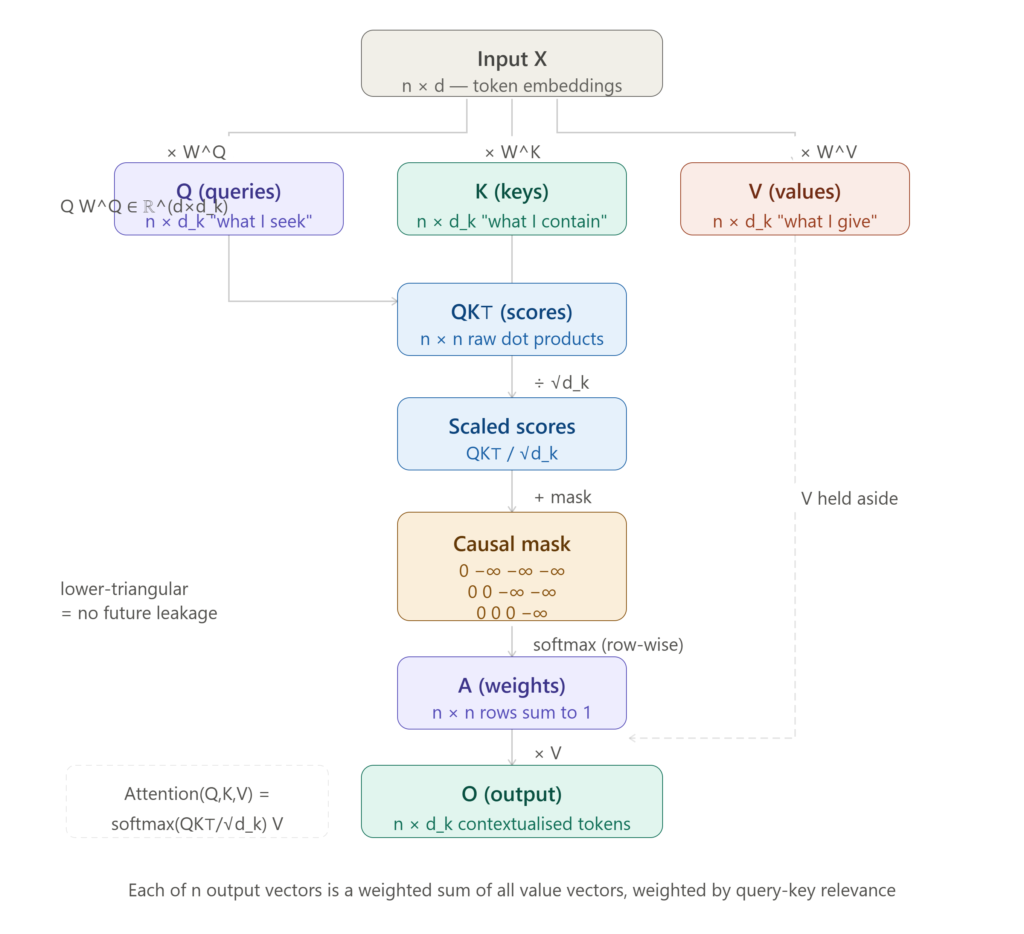
Multi-Head Attention
A single attention head computes one set of query-key-value interactions. But different aspects of meaning may require different attention patterns simultaneously: a token might need to attend to its syntactic head, its semantic antecedent, and its positional neighbours all at once. Multi-head attention runs attention operations in parallel: where are per-head projection matrices, each head operates in a dimensional subspace, and is a final output projection that mixes the concatenated heads back into the full -dimensional space.
In GPT-3, and , so each head operates in a dimensional subspace. The 96 heads learn to specialize: empirical work in mechanistic interpretability has identified heads that track syntactic subject-verb agreement, heads that copy tokens from earlier in context, heads that attend to the most recent noun phrase, and heads that implement induction — recognizing when a pattern seen earlier in the context is repeating.
The computational cost of full self-attention is , or quadratic in sequence length. For a 128K-token context window, the attention matrix alone has billion entries, making naive computation prohibitively expensive. Efficient attention variants such as Flash Attention, Sparse Attention, Sliding Window Attention address this scaling problem, which we’ll cover in Part 3 alongside the full transformer block.
The KV Cache
During inference, a decoder-only model generates one token at a time. At step , the model processes the full sequence and predicts . Without optimization, this would require recomputing the key and value matrices for all previous tokens at every step so thar cost grows as per generation.
The KV cache eliminates this redundancy. Since the key and value representations of tokens do not change between steps (they depend only on those tokens’ positions and embeddings, which are fixed once generated), they can be cached in memory and reused. At step , only the new token’s , , need to be computed; the cached and matrices from previous steps are concatenated and the attention is computed against the full cached sequence.
This reduces per-step inference cost from to in attention computation, but at the cost of memory. A KV cache for a 128K-token context with 96 heads, 128 layers, and FP16 precision occupies on the order of tens of gigabytes. Managing KV cache memory is one of the primary challenges in deploying frontier models efficiently at scale. It is why inference hardware for long-context models requires far more VRAM than a naive parameter count would suggest.
What Attention Actually Learns
It is tempting to describe attention as a mechanism that “understands” language. It is more precise, and more useful for engineering purposes, to say that attention is a differentiable, content-based memory retrieval system. The model learns, through gradient descent on the next-token prediction objective, to configure its , , matrices such that the right values get retrieved for the right queries.
The mechanism has no built-in notion of syntax, coreference, or meaning. All of that emerges from training dynamics or from the statistical regularities of billions of documents. Understanding this distinction is important for debugging model failures: when an LLM makes a coreference error or loses track of a constraint stated early in a long context, the failure mode is almost always traceable to attention weights that were distributed incorrectly, either because the training distribution underrepresented that pattern, or because the KV cache compression strategy discarded the relevant context.
Conclusion
Self-attention is the architectural innovation that made modern LLMs possible. By allowing every token to attend directly to every other token in a single parallelisable matrix operation, it solves the long-range dependency problem that defeated earlier sequential architectures. Multi-head attention extends this by learning multiple independent attention patterns simultaneously, while the KV cache makes autoregressive inference tractable at scale.
Part 3 will take the attention output and trace it through the rest of the transformer block: the feed-forward network, layer normalisation, residual connections, and the architectural choices (decoder-only versus encoder-decoder) that distinguish GPT-style models from BERT-style ones.
Coming next in the AI Engineering series is Part 3: The Transformer Block and Architecture.
-
How Large Language Models Work — Part 1: Tokenization and Embeddings
This is Part 1 of a five-part deep-dive series on the internal mechanics of large language models. This series is written for engineers, ML practitioners, and technically advanced readers. Part 1 covers tokenization and embeddings — the first two stages through which raw text becomes a mathematical object a neural network can reason over.
Why Text Must Be Transformed
Neural networks are, at their core, mathematical functions that operate on tensors, which are multi-dimensional arrays of floating-point numbers. They cannot accept raw text strings as input. Before a language model can do anything useful, it must convert a sequence of characters into a sequence of numbers. This two-step process of tokenization followed by embedding is where all LLM processing begins, and understanding it deeply is prerequisite to understanding everything that follows.
Stage 1: Tokenization
What a Tokenizer Does
A tokenizer breaks a raw string into a sequence of discrete units called tokens, and maps each token to an integer index in a fixed vocabulary. Given the input string:
"The cat sat on the mat"a tokenizer might produce the token sequence: [464, 5171, 7231, 322, 464, 8114]
Each integer is an index into a vocabulary table of size , typically between 32,000 and 100,000 entries for modern models. GPT-4 uses a vocabulary of approximately 100,277 tokens. Llama 3 uses 128,256.
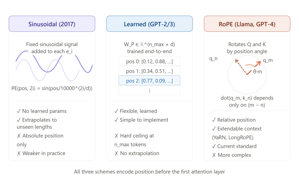
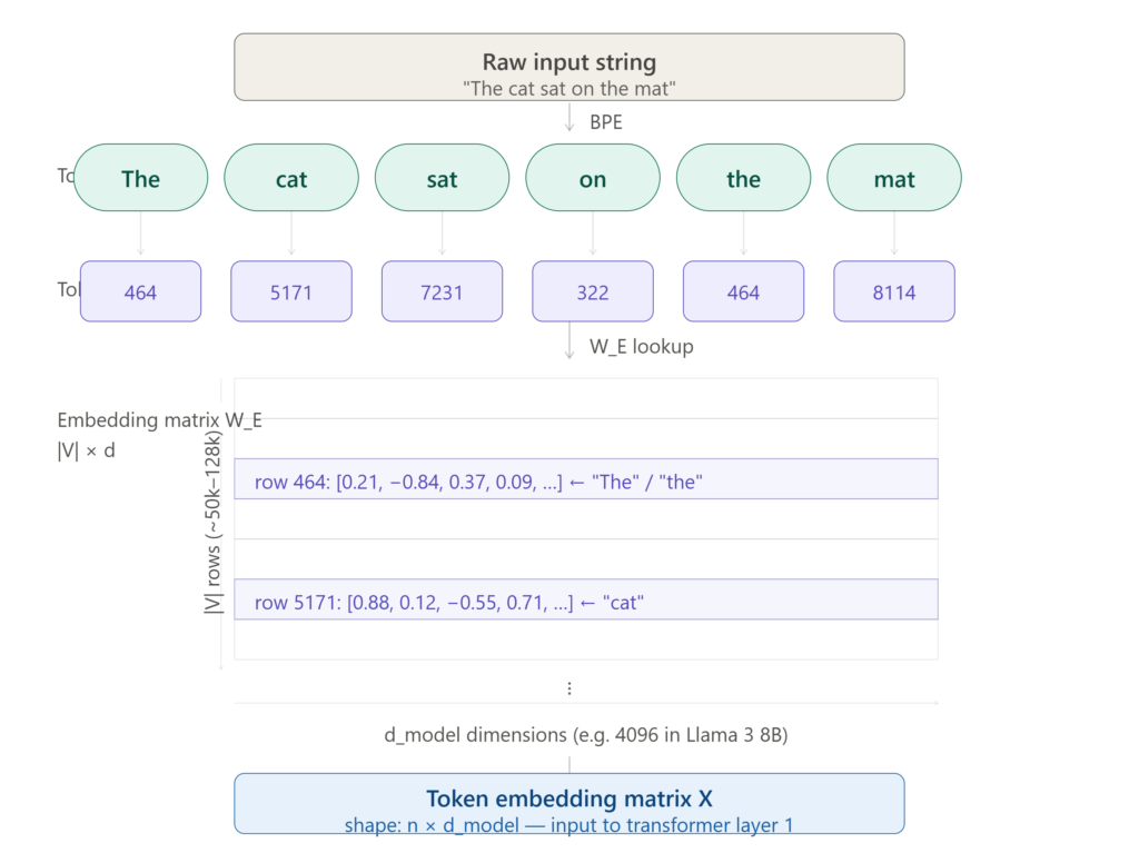
Byte-Pair Encoding (BPE)
The dominant tokenization algorithm used in modern LLMs is Byte-Pair Encoding (BPE), originally a data compression algorithm adapted for NLP by Sennrich et al. in 2016.
BPE builds its vocabulary through an iterative merging process:
- Initialise the vocabulary with every individual character (or byte) in the training corpus.
- Count all adjacent symbol pairs across the corpus.
- Merge the most frequent pair into a single new symbol.
- Repeat steps 2–3 until the vocabulary reaches the target size ∣V∣.
The result is a vocabulary that contains individual characters, common subwords, and frequent whole words. The word “tokenization” might be represented as three tokens:
token,izationis further split intoiz,ationdepending on training corpus frequency.This has a critical practical consequence: no word is ever truly unknown to a BPE tokenizer. Any string, including code, URLs, foreign scripts, or novel proper nouns, can be decomposed into its constituent bytes if nothing else matches. This is why BPE-based models generalise to inputs they have never seen verbatim.
Token Fertility and Efficiency
Not all languages tokenize equally efficiently. English text typically tokenizes at roughly 0.75 tokens per word. Languages with richer morphology, such as Finnish, Turkish, Arabic, or non-Latin scripts, tokenize less efficiently, sometimes requiring 3–5 tokens per word. This has practical implications: a context window of 128,000 tokens holds far more English prose than it does Thai or Arabic text, a bias baked into the model’s architecture from the vocabulary construction stage.
The fertility of a tokenizer, or the average number of tokens per word, is a meaningful measure of how well it serves a given language or domain. Code-optimised models like DeepSeek Coder use vocabularies with explicit code tokens to reduce the fertility of common programming constructs.
WordPiece and SentencePiece
Two notable alternatives to BPE are worth knowing:
WordPiece, used in BERT and its derivatives, is similar to BPE but merges pairs that maximise the likelihood of the training data under a language model, rather than simply the most frequent pair. This produces slightly different vocabulary distributions.
SentencePiece, used in models including Llama and T5, treats the input as a raw unicode byte stream with no pre-tokenization step (no whitespace splitting). This makes it language-agnostic and particularly well-suited for multilingual models.
Stage 2: Token Embeddings
The Embedding Matrix
Once tokenization has produced a sequence of integer indices , each index must be converted into a dense vector. This is done via an embedding matrix , where is the model’s hidden dimension (also called the embedding dimension or ).
The embedding for token ti is simply a row lookup:In GPT-3, . In Llama 3 8B, . This single matrix, learned entirely from data during pre-training, is responsible for encoding the semantic relationships between all tokens in the vocabulary.
The number of parameters in the embedding matrix alone is . For GPT-4’s approximate configuration, that is which is often hundreds of millions of parameters just for this one component.
Why Dense Vectors Work: The Geometry of Meaning
The remarkable property of learned embeddings is that semantic relationships emerge as geometric relationships in . The classic demonstration is the linear analogy:
This is not programmed. It emerges from the statistical structure of co-occurrence patterns in the training corpus. Words that appear in similar contexts end up with similar embedding vectors, measured by cosine similarity:In high-dimensional spaces, this geometry becomes extraordinarily rich. Directions in embedding space can encode syntactic roles, semantic fields, sentiment polarities, and factual associations — all simultaneously, in different orthogonal subspaces of the same .
Stage 3: Positional Encoding
Token embeddings encode what each token is, but they contain no information about where in the sequence each token appears. The sequence
"dog bites man"and"man bites dog"would produce identical sets of token embeddings in a different order and would be catastrophic for a model that needs to understand syntax and word order.Positional information must therefore be injected explicitly.
Sinusoidal Positional Encoding (Original Transformer)
The original transformer paper (Vaswani et al., 2017) proposed adding a fixed sinusoidal signal to each token embedding. For position pos and dimension i:
The input to the first transformer layer is then:
The sinusoidal formulation has a useful property: the positional encoding of position can be expressed as a linear function of the encoding at pos, which makes it easy for attention heads to learn to attend to tokens at a fixed relative offset.
Learned Positional Embeddings
GPT-2 and GPT-3 replaced sinusoidal encodings with learned positional embeddings: a second matrix , where is the maximum context length. Position pos adds the row to the token embedding. These are learned end-to-end during pre-training and tend to slightly outperform sinusoidal encodings on benchmarks, at the cost of a hard context length ceiling — the model cannot generalise beyond positions it has seen during training.
Rotary Positional Embedding (RoPE)
The current state of the art for most frontier models, including Llama, Mistral, GPT-4, and Gemini, is Rotary Positional Embedding (RoPE), introduced by Su et al. in 2021.
Rather than adding a positional vector to the token embedding, RoPE encodes position by rotating the Query and Key vectors in the attention mechanism (covered in Part 2) by a position-dependent angle. For a vector at position m in dimension pair :
where .
The critical advantage: the dot product between a query at position m and a key at position n depends only on their relative offset , not their absolute positions. This gives the model a natural inductive bias toward relative position awareness, and with extensions like YaRN makes it possible to extend the effective context window well beyond what the model was trained on.
RoPE is why modern models can be fine-tuned to handle 128K or even 1M token context windows without retraining the entire model from scratch.
Putting It Together: The Input Representation
The final input to the first transformer layer for a sequence of n tokens is a matrix :where is the positional encoding for position (sinusoidal, learned, or RoPE-derived). Each row of is a -dimensional vector carrying both the semantic identity of the token and its position in the sequence. This matrix is what flows into the self-attention mechanism, which is the subject of Part 2.
Key Numbers to Anchor Your Intuition
Model Vocabulary Positional scheme GPT-2 50,257 768–1,600 Learned GPT-3 50,257 12,288 Learned Llama 3 8B 128,256 4,096 RoPE Mistral 7B 32,000 4,096 RoPE Gemma 2 256,000 2,304–3,584 RoPE
Conclusion
Before a single attention head fires, a large language model has already done substantial mathematical work. A raw string has been segmented into subword tokens by a BPE or SentencePiece algorithm, each token has been projected into a high-dimensional vector space where geometry encodes meaning, and position information has been woven in either additively or, in modern models, rotationally via RoPE. The quality of this input representation has an outsized effect on everything downstream: models with poorly constructed vocabularies or weak embedding initialisations are harder to train and less capable at convergence.
Part 2 will take this matrix and walk through exactly what the self-attention mechanism does with it, including the full mathematical derivation of scaled dot-product attention, multi-head attention, and what different heads actually learn to represent.
Coming next in the AI Engineering series is Part 2: The Attention Mechanism.